
Abstract
Accurate channel estimation with limited pilot overhead is a key bottleneck for 6G MU-mMIMO, particularly at mmWave (with implications for THz) where path loss and multiuser interference are severe. We propose a two-stage least squares convolutional neural network (LS-CNN) framework in which a robust LS estimator provides a stable coarse channel estimate, avoiding the sparsity assumptions of compressed sensing algorithms that often fail in rich-scattering outdoor environments. In the second stage, this estimate is refined using a CNN trained on a hybrid dataset expanded through controlled augmentation of a generative adversarial network (GAN), improving generalization while minimizing pilot overhead. Training data is refined using mean squared error (MSE) thresholds to ensure high-quality samples, and a robust standardization method is used to stabilize learning with complex-valued input. Simulations on the DeepMIMO ray-tracing dataset demonstrate that the proposed approach provides an up to 8 dB normalized MSE (NMSE) improvement at low signal-to-noise ratio (SNR) over classical LS and MMSE estimators. In our experiments, it achieves performance comparable to that of the ideal MMSE estimator while requiring 60% fewer pilot symbols. Complexity analysis confirms that the proposed hybrid architecture is significantly more efficient than state-of-the-art Vision Transformers, making it practical for real-time 6G deployments.
In this article
What can a receiver learn from fewer pilots?
Pilot symbols help a receiver understand its channel, but they occupy resources that could carry data. This study first computes a coarse least-squares estimate, then refines it with a CNN trained using ray-traced and GAN-augmented data. The GAN belongs to training; inference follows the LS-to-CNN path.
Multi-user massive MIMO needs accurate channel estimates while keeping pilot overhead manageable. A classical least-squares estimate is inexpensive but noisy, especially at low signal-to-noise ratios.
From the question to the evidence
Frame the pilot-budget problem
Known pilot symbols reveal how the wireless channel transforms a signal, but they occupy resources that could carry data. The research asks whether a classical initial estimate followed by learned refinement can retain useful estimation accuracy with fewer pilots.
Channel-estimation study, pp. 1-3, Introduction and Section III. Read source · PDF page 1 ↗
Construct a physically grounded channel model
Use the outdoor DeepMIMO ray-tracing scenario, with user locations drawn from its geometric grid. The modeled uplink has a single 32-antenna base station serving 20 single-antenna users. The scenario is quasi-static within a coherence interval, and the received pilot observation combines the known pilot matrix, the channel, and additive noise.
Channel-estimation study, p. 2, Section II and Eq. (1); p. 4, Fig. 2; p. 5, Section III-C. Read source · PDF page 2 ↗
Produce the coarse least-squares estimate
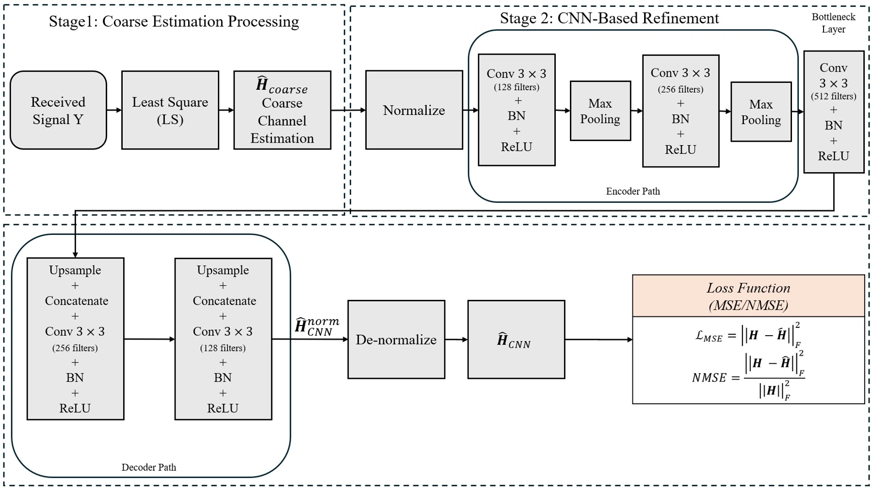
Start with a low-cost linear estimate derived from the received pilots. Algorithm 1 includes a regularization term. This initialization gives the CNN a structured channel estimate to refine instead of asking the neural model to learn the complete recovery process directly from the received waveform.
Channel-estimation study, p. 3, Section III-A; p. 4, Algorithm 1; research presentation PDF p. 13. Read source · PDF page 3 ↗ · Related presentation topic →
Prepare the offline training data
Pair coarse estimates with their ray-traced reference channels and normalize real and imaginary components. The paper retains training samples below an MSE threshold of 0.01 and reports discarding about 15%; testing uses a stricter half-threshold. These selection rules are part of the experiment and must remain visible when interpreting its results.
Channel-estimation study, pp. 4-5, Section III-C. Read source · PDF page 4 ↗
Augment and learn, before inference
A GAN learns the distribution of training-domain coarse estimates and supplies a separate augmentation branch. The refinement CNN is trained with ray-tracing and augmented data to minimize channel-reconstruction MSE. The article does not fully specify how every synthetic input is paired with a reference target; this roadmap does not invent that missing procedure.
Channel-estimation study, p. 4, Section III-B, Eqs. (8)-(9); p. 5, GAN-based data augmentation and Eq. (11). Read source · PDF page 4 ↗
Run the LS-to-CNN inference path
At inference, compute the coarse LS estimate, apply the defined normalization, refine it through the trained encoder-decoder CNN, and reverse the associated normalization to recover a channel estimate. The GAN is not called in this path.
Channel-estimation study, p. 4, Algorithm 1; p. 3, Fig. 1; research presentation PDF p. 13. Read source · PDF page 4 ↗ · Related presentation topic →
Evaluate accuracy, pilot use, and cost separately
Compare estimation NMSE over the reported 0-20 dB SNR range, inspect the pilot-count comparison at 10 dB, and report inference time alongside model size. Spectral efficiency is an additional modeled outcome. Each measure answers a different question, so lower estimation error is not treated as a measurement of end-to-end receiver reliability.
Channel-estimation study, pp. 5-6, Section IV and Figs. 3-6; research presentation PDF pp. 17-18. Read source · PDF page 5 ↗ · Related presentation topic →
Read the outcome within its scope
The paper reports a substantial low-SNR estimation improvement and a smaller pilot budget in its selected DeepMIMO evaluation. Generalization to new sites, mobility, receiver error rates, and deployment hardware requires further validation. The conclusion identifies RIS-assisted channels and alternative refinement structures as future directions.
Channel-estimation study, pp. 5-7, Sections IV-V. Read source · PDF page 5 ↗
Architecture and compact method notes
Architecture & information flow
The architecture separates linear initialization from nonlinear refinement. A least-squares stage produces a coarse complex-valued channel estimate. After normalization, an encoder uses three convolutional blocks with convolution, batch normalization, dropout, and pooling. A deeper bottleneck captures features, and a decoder upsamples with skip connections to reconstruct the channel representation. The output is returned to the channel scale through the associated inverse normalization. The separate GAN branch expands offline training data; it is not an extra receiver-stage call. The published architecture is a method description, and a reproducible implementation additionally needs unambiguous preprocessing, synthetic input-target pairing, dataset splits, and training settings.
Channel-estimation study, pp. 3-5, Fig. 1, Section III-B, Algorithm 1, and Section III-C; research presentation PDF p. 13. Read source · PDF page 3 ↗ · Related presentation topic →
- Start with received pilotsUse the received signal and known pilot matrix to compute a regularized least-squares estimate of the channel.
- Normalize the estimateStandardize the real and imaginary channel components before neural refinement.
- Refine with a CNNApply an encoder-decoder CNN with skip connections to denoise and reconstruct the channel estimate, then reverse normalization.
- Augment training separatelyTrain the refinement model on selected ray-tracing samples and GAN-augmented training data. The GAN is not an inference stage.
What the study reports
The study uses an outdoor DeepMIMO ray-tracing dataset and a single-cell setup with a 32-antenna base station and 20 users. Evaluation spans SNR values from 0 to 20 dB. Samples are filtered by reconstruction-error thresholds; results apply to that reported evaluation pipeline.
These are results reported by the source publication, not an independent reproduction. Conditions and source disagreements are retained beside the evidence they affect.
These are the study's modeled conditions, not a specification for a live deployment.
| Setting | Reported configuration |
|---|---|
| Channel source | Outdoor DeepMIMO ray-tracing scenario |
| Network model | Single-cell, centralized, quasi-static uplink |
| Base-station antennas | 32 |
| Users | 20, each with one antenna |
| SNR range for the NMSE comparison | 0 to 20 dB |
| SNR for the pilot-count comparison | 10 dB |
Channel-estimation study, p. 2, Section II; p. 4, Fig. 2; pp. 5-6, Section IV-A/IV-C and Figs. 3/5. Read source · PDF page 2 ↗
Users are sampled from the ray-tracing scenario's geometric grid. The selected propagation environment and data preparation constrain the interpretation of the comparison.
MSE filtering is a sample-selection rule. Its threshold is not the same quantity as the NMSE-in-dB values used to report performance.
| Data preparation item | Reported rule |
|---|---|
| Training-sample retention | MSE below 0.01 |
| Discarded training samples | About 15% |
| Testing threshold | Half the training threshold, described as stricter |
| CNN training objective | Unnormalized channel-reconstruction MSE |
| Reported accuracy metric | NMSE in dB |
Channel-estimation study, p. 4, Eqs. (9)-(10); p. 5, Section III-C. Read source · PDF page 4 ↗
Testing on a more tightly selected subset conditions the reported outcome. These figures do not establish performance on every channel sample or on an independently deployed receiver.
Outdoor DeepMIMO evaluation under the reported sample-selection procedure. More negative NMSE indicates lower normalized estimation error.
| Reported method or comparison | NMSE result at SNR = 0 dB |
|---|---|
| Proposed framework | Approximately -14.2 dB |
| LS / MMSE baseline | Approximately -6.0 dB |
| Improvement summarized in the article | About 8 dB |
Channel-estimation study, p. 5, Section IV-A; p. 6, Fig. 3. Read source · PDF page 5 ↗
These values are explicitly stated in the article, not estimated from graph pixels. The prose groups the proposed hybrid/standalone framework; the website does not infer a separate numeric gain from GAN augmentation alone.
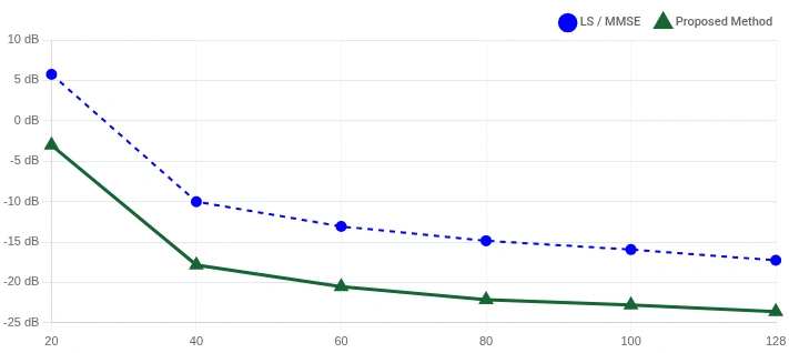
The paper presents the 40-pilot result as comparable to the baseline at 128 pilots. The original curve is available in the accompanying presentation figure.
| Item | Reported value or observation |
|---|---|
| Comparison SNR | 10 dB |
| Proposed pilot count highlighted in the source | 40 pilot symbols |
| Baseline count cited for the comparison | 128 pilot symbols |
| NMSE at 40 pilots in the figure caption | -17.8 dB |
| NMSE at 40 pilots in the adjacent prose | Approximately -16 dB |
Channel-estimation study, pp. 5-6, Section IV-C and Fig. 5; research presentation PDF p. 17. Read source · PDF page 5 ↗ · Related presentation topic →
This table makes the source discrepancy visible: the caption and prose give different errors at 40 pilots, and the printed percentage does not agree with the stated pilot counts. No resolved percentage, exact equivalence, or new curve data is asserted.
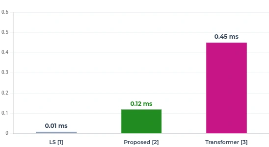
Times and parameter counts are taken from the study's own comparison. The source does not provide enough hardware, batching, or repetition information to reproduce a portable latency benchmark.
| Estimator | Time per sample | Reported trainable parameters |
|---|---|---|
| Least squares | 0.01 ms | Not a trained neural model |
| Proposed U-Net refinement model | 0.12 ms | Approximately 8.35 million |
| Transformer baseline | 0.45 ms | Approximately 0.34 million |
Channel-estimation study, p. 5, Transformer baseline description; p. 6, Section IV-D and Fig. 6; research presentation PDF p. 18. Read source · PDF page 5 ↗ · Related presentation topic →
The CNN is larger by parameter count but has a lower reported sample time than the configured Transformer. This is a size-versus-runtime trade-off in the source, not evidence that every CNN is smaller or faster than every Transformer.
This approximate value is reported in the performance-summary prose; it is not a new value digitized from the curve.
| Outcome | Value stated in the article | Condition |
|---|---|---|
| Proposed estimator's spectral efficiency | Approximately 23 bit/s/Hz | SNR = 20 dB |
Channel-estimation study, p. 5, Section IV-B; comparison figure on p. 6, Fig. 4. Read source · PDF page 5 ↗
The plotted rates and reported NMSE are separate evaluation quantities. They do not by themselves measure bit-error rate, decoding reliability, or end-to-end network throughput in a live system.
Additional reported observations
- At SNR = 0 dB, the paper reports approximately -14.2 dB NMSE for its proposed framework, compared with -6.0 dB for the LS/MMSE baseline: about an 8 dB difference in this experiment.
Channel-estimation study, PDF p. 5, Section IV-A; Fig. 3 on p. 6. Read source · PDF page 5 ↗
- The study reports comparable estimation accuracy with a smaller pilot budget. An exact percentage is not repeated here because the figure caption, pilot counts, and prose are inconsistent.
Channel-estimation study, PDF pp. 5-6, Section IV-C and Fig. 5. Read source · PDF page 5 ↗
Inspect the source figures
Read the original presentation visuals with their evaluation conditions. Open a figure to inspect its labels and axes.
Scope & limitations
- Performance is reported on a selected ray-tracing dataset, not a live network deployment.
- The dataset-generation section filters training examples by MSE and applies a stricter threshold at testing; this conditions how the reported accuracy should be interpreted.
- The pilot-reduction percentage and pilot counts differ within the supplied paper. The site preserves the original abstract while avoiding that percentage as a standalone claim.
- Lower estimation error does not establish end-to-end receiver reliability in every propagation condition.
- Inference timings are study-specific and lack sufficient hardware context for a general speed guarantee.
Cited in context
Survey discussion and comparison
A Survey of Intelligent Methods Under Inadequate Pilots in 5G/6G MIMO Systems: Pilot-Domain Mitigation, Channel Estimation, and Receiver Processing
The survey discusses LS-to-U-Net channel refinement and GAN-augmented offline training as one approach to limited-pilot channel estimation. Its comparison also notes the paper's reported spectral-efficiency evaluation.
This is a review of the method and its reported results. It does not constitute an independent reproduction, a collaboration, or an endorsement.
Inspect reference [40] →Method outline
Educational adaptation of Algorithm 1, not executable research code or a validated reproduction. The preprocessing specification includes the normalization and inverse transformation needed at inference; its fitted parameters and deployment protocol are not supplied here. Offline GAN augmentation belongs to model preparation and is deliberately outside this inference sequence.
Conceptual inference pseudocode · pseudocode
INPUT: received pilot observations, known pilot matrix
INPUT: trained refinement CNN and defined preprocessing

COARSE ESTIMATE ← regularized least-squares initialization
NORMALIZED ESTIMATE ← normalize the coarse estimate
REFINED REPRESENTATION ← apply the trained CNN
CHANNEL ESTIMATE ← reverse the associated normalization

RETURN the refined channel estimate

OFFLINE ONLY: ray-tracing data and GAN augmentation
support training of the refinement modelChannel-estimation study, p. 4, Algorithm 1; p. 5, Section III-C; research presentation PDF p. 13. Read source · PDF page 4 ↗ · Related presentation topic →
Presentation guide and further interpretation
Read the architecture from left to right
The diagram on presentation PDF page 13 follows the coarse-estimate and refinement stages. Locate the LS block first, then normalization, the encoder-decoder, and the output transform. Treat this as the inference path; read the separate training explanation to understand where GAN augmentation enters.
research presentation PDF p. 13; Channel-estimation study, p. 3, Fig. 1, and p. 4, Algorithm 1. Read source · PDF page 3 ↗ · Related presentation topic →
Read the pilot curve as a fixed-SNR comparison
Presentation PDF page 17 plots the number of pilots horizontally and NMSE in dB vertically, with SNR fixed at 10 dB. Compare the two curves at the same pilot count. The result supports the study's smaller-budget narrative, while the accompanying evidence table preserves the conflicting point descriptions instead of silently choosing one.
research presentation PDF p. 17; Channel-estimation study, p. 6, Fig. 5. Read source · PDF page 6 ↗ · Related presentation topic →
Read the timing bars together with model size
Presentation PDF page 18 reports per-sample time for LS, the proposed estimator, and the Transformer baseline. The table pairs these timings with the paper's parameter counts. This reveals the reported computational trade-off without turning a source-specific measurement into a hardware-independent speed claim.
research presentation PDF p. 18; Channel-estimation study, p. 6, Section IV-D and Fig. 6. Read source · PDF page 6 ↗ · Related presentation topic →
Further interpretation notes
- All numerical results here are author-reported study values. The website does not execute the research implementation or claim an independent reproduction.
- GAN augmentation and the CNN's deployment path are distinct. The source does not fully specify synthetic input-target pairing, so no such procedure is invented in the pseudocode.
- Training and test sets are selected using different reconstruction-error thresholds. The low-SNR numbers must be interpreted within that filtering procedure.
- The source's pilot-search interval and its plotted pilot counts are not fully consistent; the website does not present the described search as a reproduced or certified optimal pilot-selection algorithm.
- Figure 5 and its adjacent prose differ on NMSE at 40 pilots. The source's percentage reduction also conflicts with its stated counts; the published abstract remains unchanged, while these explanations expose the ambiguity.
- Reported inference times lack hardware and batch context. Model size, runtime, estimation accuracy, and receiver reliability are different quantities.
- No additional SNR-curve samples, confidence intervals, error bars, training-set sizes, latency distributions, or speed ratios are synthesized from the figures.
Cite this article
Pooya Hejazi; Masoud Sabaei; Ali Hajmahmoudi. (2026). Pilot-Efficient Channel Estimation for 6G MU-mMIMO Using LS Initialization and GAN-Augmented CNN Refinement. Journal of Communications and Networks, 28(3), 401–408. https://doi.org/10.23919/JCN.2025.000112
BibTeX
@article{Hejazi2026ChannelEstimation,
  title = {Pilot-Efficient Channel Estimation for 6G MU-mMIMO Using LS Initialization and GAN-Augmented CNN Refinement},
  author = {Hejazi, Pooya and Sabaei, Masoud and Hajmahmoudi, Ali},
  journal = {Journal of Communications and Networks},
  year = {2026},
  volume = {28},
  number = {3},
  pages = {401--408},
  doi = {10.23919/JCN.2025.000112},
  url = {https://doi.org/10.23919/JCN.2025.000112}
}Download BibTeX · Download RIS
Article © its authors. CC BY-NC 3.0. Original PDF and rights notices preserved.