Presentation atlas

Research, explained.

Explore the complete presentation, from the first research question to the final conclusions.

Each visual is paired with an English explanation of the idea, the method, and the evidence. Expand a topic to read more, or open its image for a closer look.

Complete collection

Foundations

Learning to estimate channels and allocate radio resources

White title page with a navy research title, author and advisor details, a blue vertical rule, and the Amirkabir University of Technology emblem.
Learning to estimate channels and allocate radio resources. Source: Pooya Hejazi’s research presentation. Open image to inspect.

Pooya Hejazi's research presentation brings together two connected questions in wireless systems: how to recover useful channel information from limited pilots, and how to translate channel conditions into user groups and radio-resource assignments. The programme combines mathematical models with learning methods at these different decision levels.

Research scope

The channel-estimation study starts with a classical least-squares estimate and learns a refinement using a convolutional network. A separate generative model supports training-data augmentation. The user-clustering study first formulates resource allocation mathematically, then uses optimization-derived labels to train a neural predictor.

Read the full explanation

Academic context

The presentation names Pooya Hejazi as its author and Masoud Sabaei as advisor, within the Department of Computer Engineering at Amirkabir University of Technology. These details describe the supplied academic material. The two corresponding journal records provide the authoritative publication titles, author lists, and publication dates.

How to use the collection

Follow the sequence for a guided account of motivation, assumptions, architecture, evaluation, and research directions. Read each figure together with its English explanation: the original presentation is preserved, while the notes distinguish reported findings, explanatory diagrams, and statements that the associated papers do not establish.

Technical details

  • The title frames prospective 6G research; it does not describe a deployed commercial network.
  • The presentation's academic date is retained in the original image without inferring a degree-conferral date.

Further reading: Supplied doctoral presentation, title and research outline. · Paper 2, Introduction and Conclusion. · Paper 1, Introduction and Conclusion.
Foundations

A route through the research

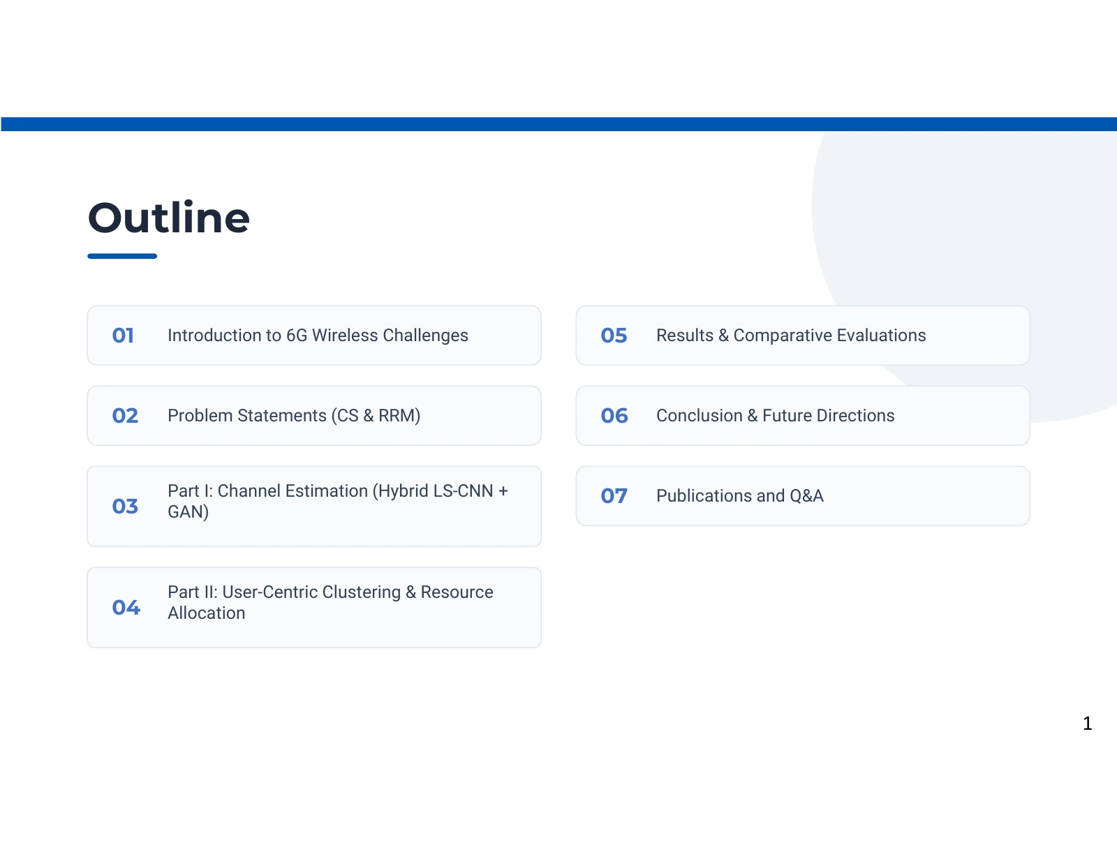
Seven rounded outline items arranged in two columns, covering motivation, two research parts, evaluation, conclusions, and publications.
A route through the research. Source: Pooya Hejazi’s research presentation. Open image to inspect.

The presentation moves from wireless-system requirements to two specific research problems, then follows each method into its results and limitations. This outline helps readers connect a technical component to the question it answers, and keeps channel estimation distinct from user clustering and resource allocation.

Two complementary questions

The first part concerns the physical channel: a receiver observes known pilots and estimates the channel coefficients needed for subsequent processing. The second concerns network decisions: users must be grouped and assigned radio resources under the modeled constraints.

Read the full explanation

From method to evidence

Architectures explain how information moves through a method. The result panels then ask different questions about estimation error, pilot requirements, runtime, or spectral efficiency. These quantities should be read separately before considering their trade-offs.

A reading convention

English notes accompanying the original visuals identify the relevant paper and explain the conditions attached to numerical claims. A presentation illustration is not automatically a published experiment, and a shared research theme does not establish that both methods were tested as one integrated system.

Technical details

  • The two principal journal articles are linked independently throughout the collection.

Further reading: Supplied doctoral presentation, research outline. · Paper 2, Sections II–V. · Paper 1, Sections II–V.

Foundations

Why future wireless systems need efficient inference

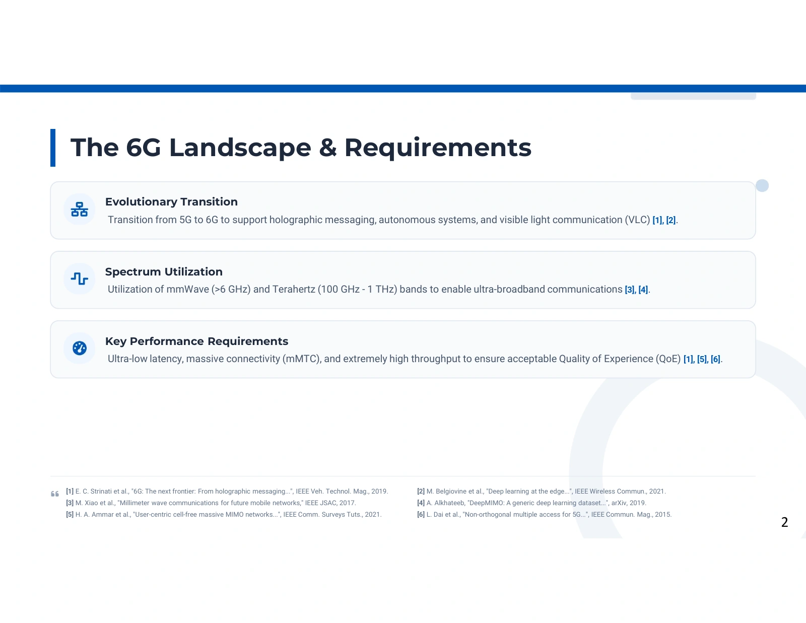
Three horizontal cards about the evolution toward 6G, spectrum utilization, and latency, connectivity, and throughput requirements, with short reference entries below.
Why future wireless systems need efficient inference. Source: Pooya Hejazi’s research presentation. Open image to inspect.

Three panels connect anticipated applications, wider spectrum use, and demanding service requirements. Their purpose is to motivate research on channel knowledge and resource management: a large antenna system must learn enough about its environment to communicate efficiently, while its control decisions must remain computationally practical.

Applications create competing demands

The applications named in the presentation are examples of the broader research motivation. High data rates, many connected devices, and short response times put pressure on different parts of a communication system. Improving one local measure does not automatically satisfy them all: more training pilots can improve channel estimation while consuming transmission resources that might otherwise carry data.

Read the full explanation

Why channel knowledge matters

Multiple antennas offer spatial degrees of freedom, but exploiting them requires knowledge of how signals propagate between transmitters and receivers. The estimation article therefore focuses on recovering channel coefficients economically. The clustering article addresses another use of channel information: selecting user groups and serving resources that support a favorable modeled sum-rate.

Separate the vision from the experiment

The spectrum ranges and application examples are background labels in the presentation. They do not establish that the experiments cover every cited band or service. The published channel-estimation comparison uses a specified outdoor DeepMIMO model; the clustering paper uses its own modeled network and assumptions. Neither result is a demonstration of a complete 6G service or a certification against a system requirement.

Technical details

  • CSI means channel state information; it describes the propagation channel used by communication algorithms.
  • The spectrum labels in the image are simplified motivation, not a formal definition of frequency bands.

Further reading: Paper 2, Introduction and Section II. · Paper 1, Introduction and Section II. · Supplied doctoral presentation, wireless requirements overview.

Foundations

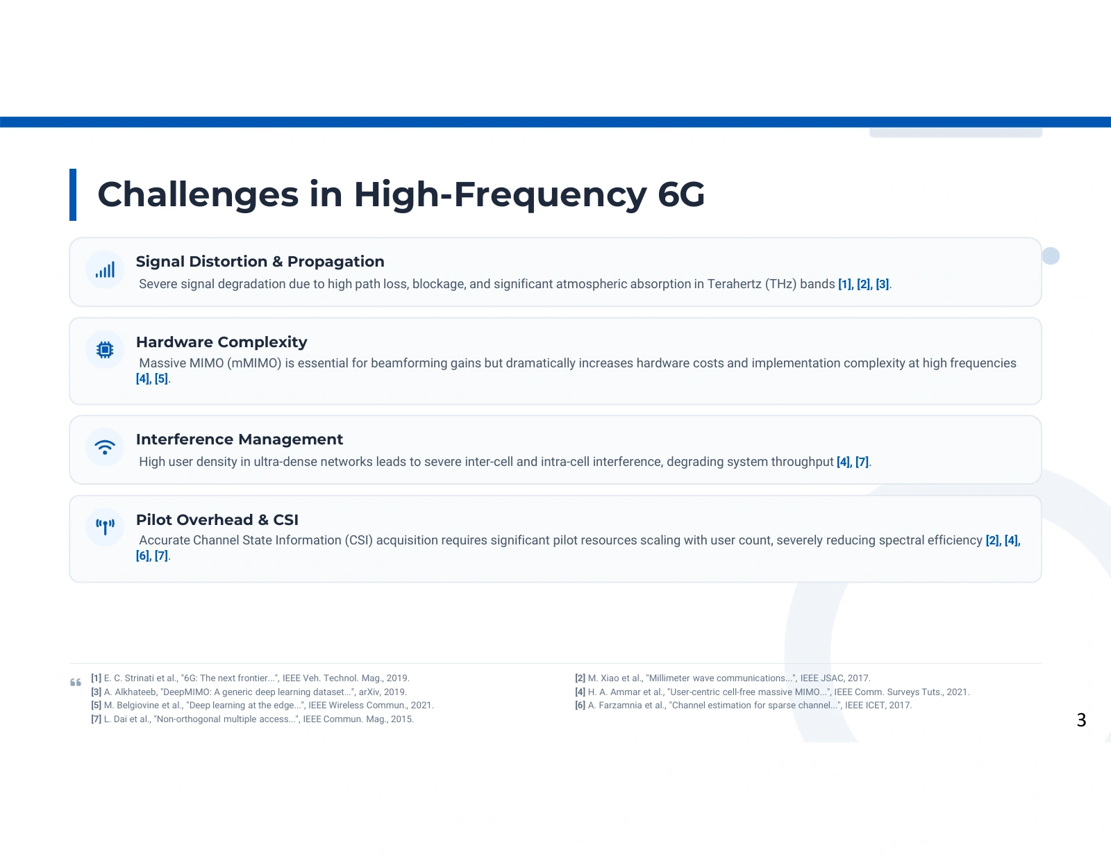
Propagation, interference, and the cost of channel knowledge

Four stacked cards identify signal distortion and propagation, hardware complexity, interference management, and pilot overhead with channel state information.
Propagation, interference, and the cost of channel knowledge. Source: Pooya Hejazi’s research presentation. Open image to inspect.

The challenge map links propagation difficulty, antenna-system complexity, interference, and pilot overhead. These pressures explain why the research treats signal recovery and resource decisions as separate technical problems. Each method addresses a part of this map under specified assumptions; neither removes every limitation shown.

Read the challenges as a dependency chain

Propagation changes the amplitude and phase of received signals. Antenna arrays can help direct or separate transmissions, but their processing depends on channel information. As more users and resources interact, interference management becomes a network decision as well as an estimation problem. The presentation uses this chain to move from a broad wireless vision to concrete algorithmic questions.

Read the full explanation

Where the proposed methods intervene

The LS–CNN estimator intervenes at channel recovery: known pilots produce a coarse estimate that a learned network refines. The clustering method intervenes at allocation: channel-dependent rates enter a constrained objective, and a predictor learns decisions from optimization-derived labels. Reducing estimation error and selecting favorable allocations are complementary objectives, with different inputs, outputs, and evaluation measures.

Assumptions determine what is demonstrated

The papers simplify the environment to make these questions tractable, including quasi-static channel models and specified interference or receiver assumptions. Their results should not be extended directly to arbitrary mobility, synchronization errors, hardware impairments, or atmospheric conditions. A successful comparison within a selected scenario establishes evidence for that scenario; deployment requires checking the omitted effects and their interaction with the learned model.

Technical details

  • A coherence interval is the period or block over which the channel is treated as approximately unchanged.
  • Pilot overhead is a resource cost; it is not an inference-time measurement.

Further reading: Paper 2, Sections I–II and IV. · Paper 1, Introduction and Section II. · Supplied doctoral presentation, high-frequency challenges.

Channel estimation

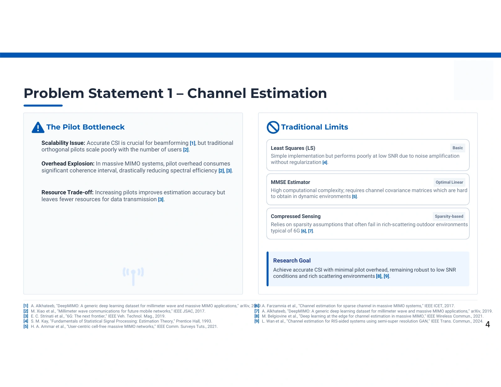
The channel-estimation problem: accuracy within a pilot budget

Two columns contrast the pilot bottleneck with least squares, MMSE, compressed sensing, and the proposed research goal.
The channel-estimation problem: accuracy within a pilot budget. Source: Pooya Hejazi’s research presentation. Open image to inspect.

A receiver needs known reference signals to infer the wireless channel, but those pilots occupy a finite transmission budget. This problem statement compares classical estimation approaches and motivates a hybrid design: retain an interpretable least-squares starting point, then learn a refinement that can be useful with fewer pilots.

What the pilot trade-off means

Pilots are known symbols used to relate the transmitted signal to the received observation. Their number and structure affect how much channel information can be recovered in noise. Spending more of a coherence block on pilots can leave less of it for payload data. The research question is therefore about useful accuracy at a smaller training budget, not simply the lowest possible error without resource constraints.

Read the full explanation

Why combine a classical and a learned estimator

Least squares recovers an initial channel estimate directly from the observation model. Its performance depends on noise, pilot design, and numerical conditioning. Statistical estimators such as MMSE use additional distributional information; sparse recovery methods exploit a chosen sparse representation. The proposed CNN refines the coarse LS representation rather than replacing every stage of channel recovery with an unconstrained learned mapping.

How the question is evaluated

The associated paper reports NMSE across a 0–20 dB SNR range and a separate pilot-count comparison at 10 dB. These experiments use a selected outdoor DeepMIMO dataset and explicit sample filtering. The useful conclusion is conditional: the hybrid estimator improves reported estimation behavior within this setup. A universal claim that LS fails, MMSE is impractical, or sparse methods cannot handle outdoor channels would go beyond the comparison.

Technical details

  • Lower NMSE means a smaller estimation error relative to the reference channel energy.
  • The pilot-count comparison contains conflicting source annotations; its detailed discussion keeps those differences visible.

Further reading: Paper 2, Introduction, Sections II–III, and Section IV-A/IV-C. · Supplied doctoral presentation, channel-estimation problem statement.

User clustering

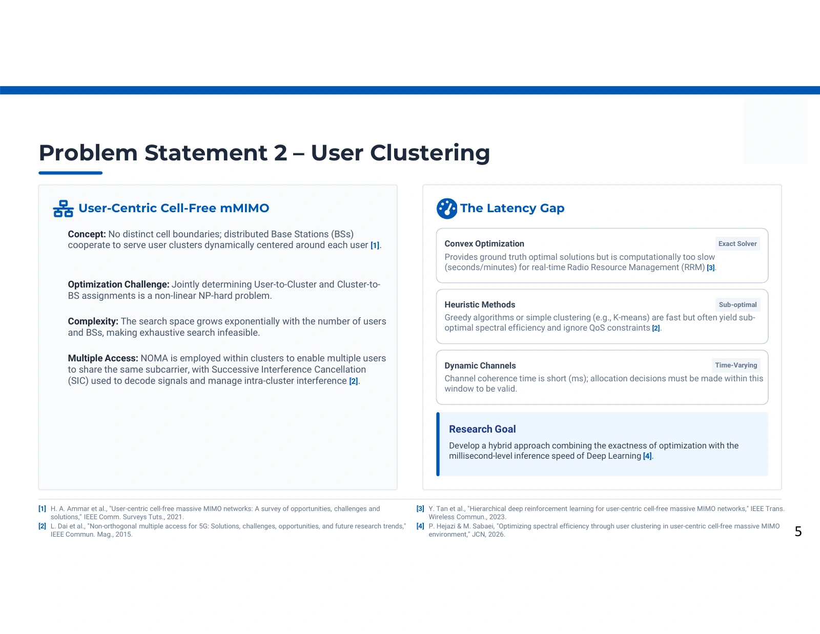
The clustering problem: useful decisions before conditions change

Two columns describe user-centric cell-free massive MIMO and a latency gap between optimization, heuristics, and decisions under changing channels.
The clustering problem: useful decisions before conditions change. Source: Pooya Hejazi’s research presentation. Open image to inspect.

The network-level problem asks which users should share clusters and which base-station resources should serve them. These are coupled discrete decisions. The proposed strategy moves a substantial part of the optimization effort into offline label generation, then learns a faster mapping from channel conditions to candidate assignments.

Why the assignment space becomes difficult

A change in group membership changes who shares resources and which interference terms matter. A change in a serving base station or subcarrier changes the rates associated with that group. The paper combines these effects in an allocation model with binary decision variables. Evaluating a large number of possible combinations can therefore be expensive even before considering deployment constraints.

Read the full explanation

The role of optimization-supervised learning

The study uses a linearized optimization formulation to generate labels for its training instances. A multilayer perceptron ensemble learns the relationship between channel gains and allocation decisions, with penalties intended to discourage constraint violations. This shifts computation in time: solving training cases and fitting the model occur offline, whereas a trained network proposes allocations during inference.

What the latency argument does not prove

Linearization does not remove integer decisions or establish that every transformed instance is a simple convex problem. Learned outputs also need explicit feasibility assessment: a loss penalty and rounded predictions do not guarantee every physical constraint. The presentation's seconds-versus-milliseconds language explains the motivation, but a portable speed claim requires solver settings, model size, hardware, and comparable workloads. The paper's objective and prediction metrics should be read alongside these limitations.

Technical details

  • UC-CF abbreviates user-centric cell-free; NOMA allows modeled resource sharing within a cluster.
  • SIC means successive interference cancellation, whose decoding assumptions are part of the rate model.

Further reading: Paper 1, Section II, Section III, and Section IV. · Supplied doctoral presentation, user-clustering problem statement.

Foundations

Three method contributions across two studies

Three horizontal contribution cards summarize LS–CNN with GAN augmentation, linearized optimization for labels, and a constraint-aware MLP ensemble.
Three method contributions across two studies. Source: Pooya Hejazi’s research presentation. Open image to inspect.

The contribution panel combines one channel-estimation contribution with two stages of the clustering study: optimization-based label generation and learned allocation. Read it as a map of the research programme. The numerical callouts require their own experiment conditions and should not be interpreted as an integrated system benchmark.

A hybrid estimator with a distinct training branch

The first contribution keeps least-squares recovery at the input and uses a CNN to refine the channel estimate. GAN augmentation belongs to training. The associated article reports approximately −14.2 dB NMSE at 0 dB SNR, with an improvement of about 8 dB relative to the classical comparison described in its prose. That is an estimator result within the selected dataset.

Read the full explanation

A model for producing allocation labels

The second contribution formulates user grouping and resource assignment with explicit variables and constraints, then applies linearization techniques to obtain training solutions. These labels give supervised learning a task-specific target. Their value depends on the accuracy of the formulation, the approximation, and the solver outcome; calling every label an exact optimum of the original nonlinear system would erase these distinctions.

A predictor intended to reduce online computation

The third contribution uses an ensemble MLP and constraint penalties to predict allocations from channel information. The relevant questions include assignment accuracy, objective-value error, feasibility, and computational cost. The displayed operation-count expression is not a measured GPU latency. Similarly, the pilot-reduction percentage belongs to the estimation study and conflicts with its stated counts; it cannot serve as a cross-study measure of network efficiency.

Technical details

  • The cited channel-estimation paper has three authors: Pooya Hejazi, Masoud Sabaei, and Ali Hajmahmoudi.
  • The allocation paper is authored by Pooya Hejazi and Masoud Sabaei.

Further reading: Paper 2, Sections III–IV, especially Section IV-A/IV-C. · Paper 1, Sections II and IV. · Supplied doctoral presentation, research contributions.

Channel estimation

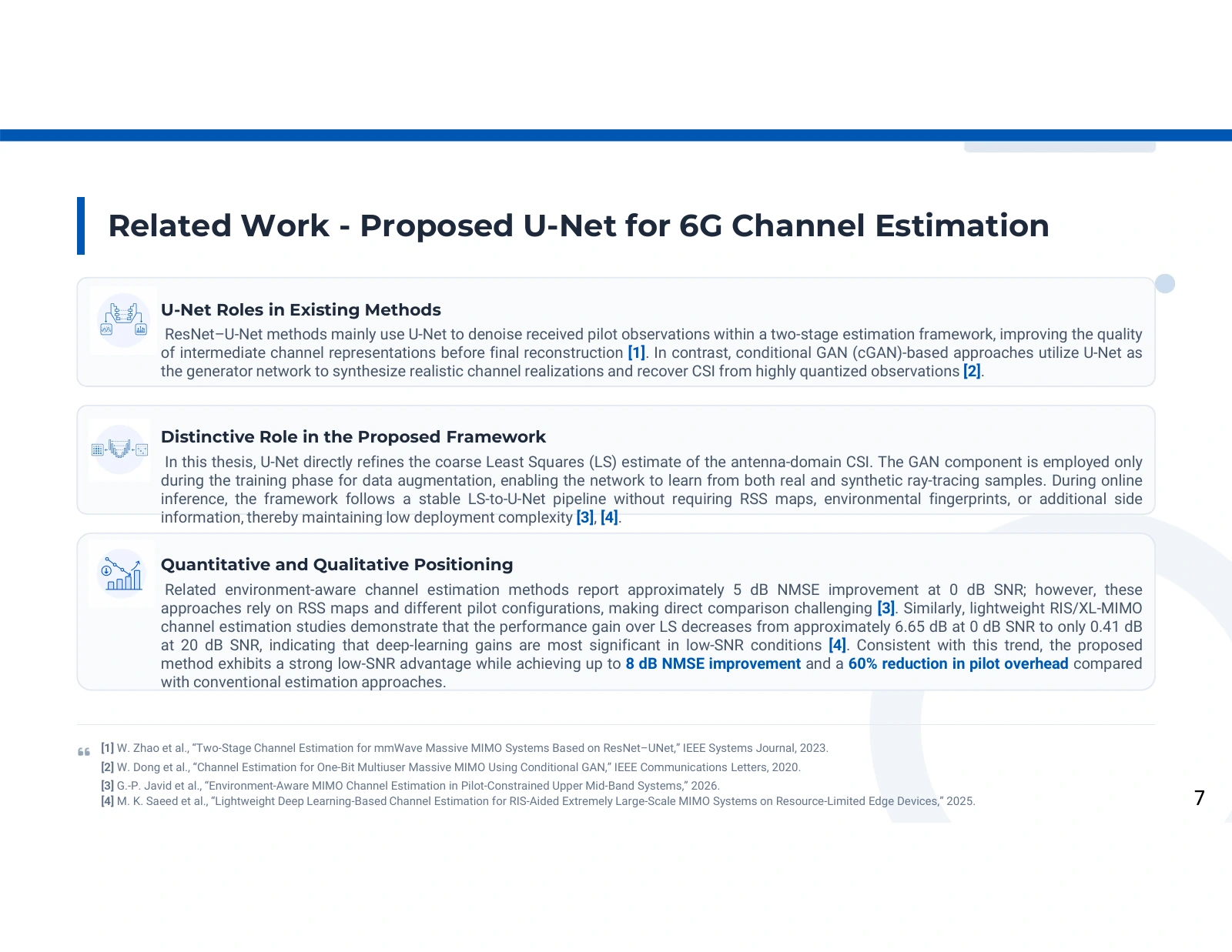
Where U-Net refinement fits among learning approaches

Three text panels compare U-Net roles in prior methods, its role in the proposed framework, and quantitative positioning, with four bibliography entries below.
Where U-Net refinement fits among learning approaches. Source: Pooya Hejazi’s research presentation. Open image to inspect.

The related-work comparison is most useful for understanding what a network receives and predicts. U-Net can denoise an observation, act as a generative component, or refine an existing estimate. Here its role is to improve a coarse antenna-domain LS estimate, while GAN augmentation supports offline training.

Distinguish the role from the architecture name

An encoder–decoder with skip connections can appear in several estimation pipelines without those pipelines solving exactly the same task. The important distinctions are the input representation, the target output, available side information, and training objective. The presentation positions this method around coarse channel estimates rather than environmental maps or a received-signal reconstruction task alone.

Read the full explanation

Follow the proposed information path

Known pilots and received observations first produce an LS estimate. The refinement network processes a normalized representation and returns an improved estimate on the channel scale. The generative model supplies training examples in an offline branch. This separation explains why the online receiver path can remain LS followed by CNN inference even though adversarial training is part of model preparation.

Compare studies only under compatible conditions

The image quotes gains from other publications, but those studies use different systems, inputs, and pilot configurations. Their numbers are background context, not a controlled leaderboard against the present experiment. The website therefore grounds its numerical conclusions in the associated paper's own comparison. An overall low-SNR gain also cannot be assigned entirely to GAN augmentation without an adequately specified and matched ablation.

Technical details

  • The external numerical comparisons are transcribed in the preserved source image; their full experimental equivalence has not been verified.
  • Paper 2 describes MSE-based CNN training and NMSE evaluation as separate quantities.

Further reading: Paper 2, Introduction, Section III-B/III-C, and Section IV. · Supplied doctoral presentation, related work on U-Net channel estimation.

User clustering

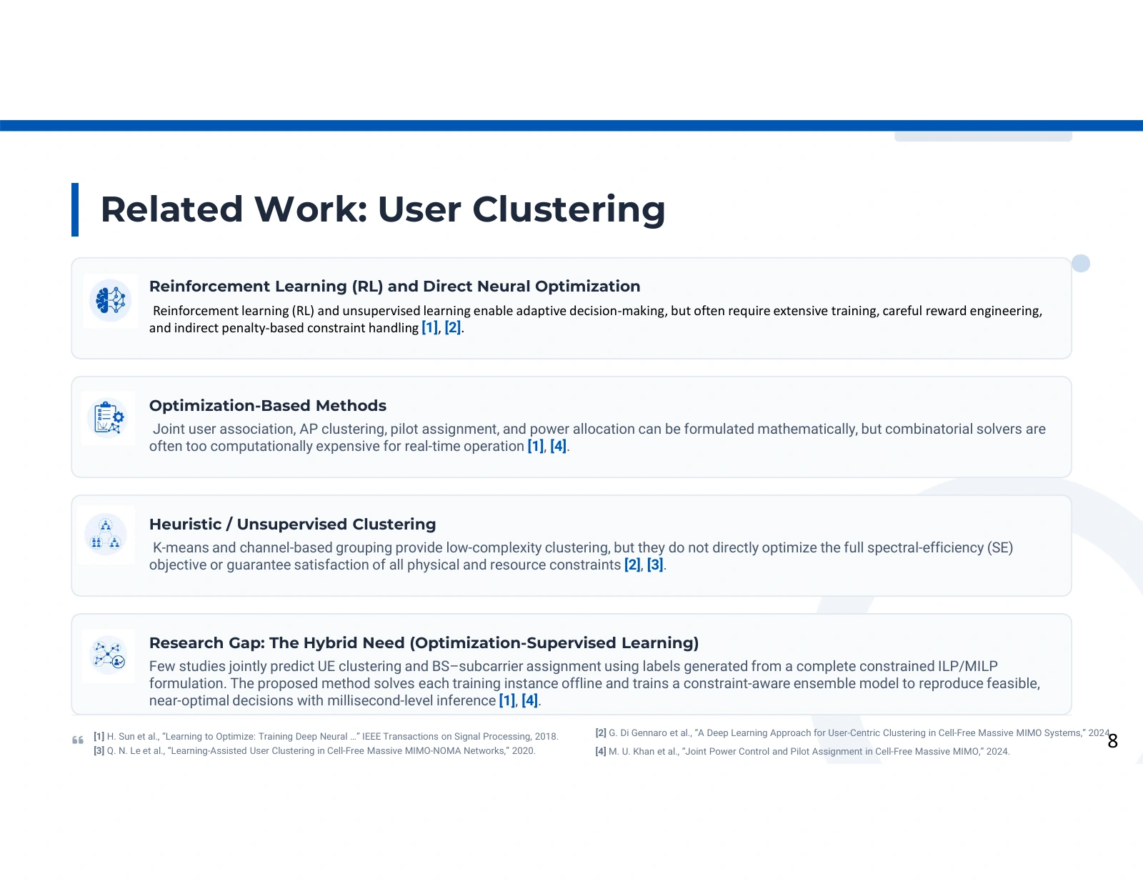
Why learn from an allocation model

Four stacked text panels compare reinforcement learning, optimization, heuristic clustering, and optimization-supervised learning; short reference entries run along the lower edge.
Why learn from an allocation model. Source: Pooya Hejazi’s research presentation. Open image to inspect.

This comparison separates reinforcement learning, mathematical optimization, heuristic grouping, and supervised prediction. The proposed approach uses optimization solutions as training targets. Its distinguishing design choice is the origin of those labels and the structure of the predicted assignments, rather than a general claim that one learning family is always superior.

Different methods encode the goal differently

An optimization model states an objective and constraints explicitly. A reinforcement-learning system depends on the environment, reward, and training procedure. A clustering heuristic may organize users by similarity without optimizing the complete communication objective. These are useful distinctions, but each category contains many methods; a short overview cannot establish the quality or limitations of every possible implementation.

Read the full explanation

The proposed supervised route

The user-clustering paper generates assignment labels by solving its linearized formulation for training channel instances. Its neural model then learns to predict user membership and base-station/subcarrier decisions. Constraint penalties connect the learned outputs to the allocation rules. This approach aims to preserve useful structure from the optimization problem while reducing the repeated computation needed to produce an online candidate.

Evidence needed to support the comparison

A meaningful assessment should distinguish label quality, prediction accuracy, achieved objective value, constraint satisfaction, and inference cost. Agreement with a solver label does not by itself prove optimality of the underlying physical network. The presentation's broad research-gap wording and descriptions of external methods are literature context; the published study's own assumptions and evaluation are the basis for this website's claims.

Technical details

  • The supplied bibliography identifies H. Sun et al., “Learning to Optimize: Training Deep Neural …,” IEEE Transactions on Signal Processing, 2018; the title is abbreviated in the source.
  • It also lists G. Di Gennaro et al., “A Deep Learning Approach for User-Centric Clustering in Cell-Free Massive MIMO Systems,” 2024; Q. N. Le et al., “Learning-Assisted User Clustering in Cell-Free Massive MIMO-NOMA Networks,” 2020; and M. U. Khan et al., “Joint Power Control and Pilot Assignment in Cell-Free Massive MIMO,” 2024.

Further reading: Paper 1, Introduction and Sections II–IV. · Supplied doctoral presentation, related work on user clustering.

Foundations

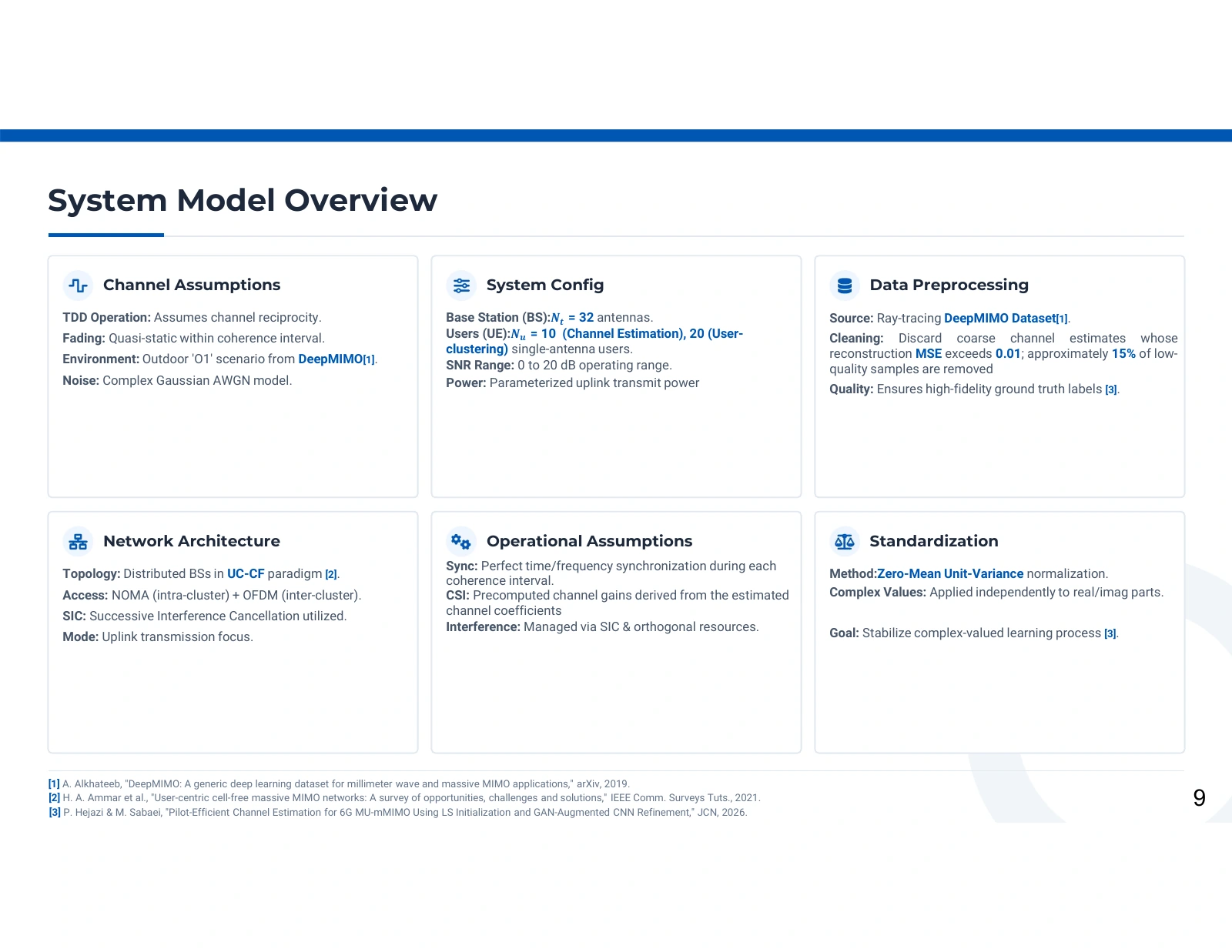
System assumptions and the boundary between the experiments

Six cards in a three-by-two grid describe channel assumptions, system configuration, data preprocessing, network architecture, operational assumptions, and standardization.
System assumptions and the boundary between the experiments. Source: Pooya Hejazi’s research presentation. Open image to inspect.

The six-panel overview combines channel, network, preprocessing, and operational assumptions. It is a useful checklist for interpreting the methods, but it merges two different experiments and contains conflicting user counts. The article-specific configurations below should guide scientific comparisons rather than treating this page as one shared simulation specification.

Separate the physical models

The channel-estimation article describes a centralized uplink with one 32-antenna base station and 20 single-antenna users. The clustering study describes a distributed network and reports 110 scenarios containing 10 users each, with five base stations and 32 antennas per base station. The overview's labels of 10 estimation users and 20 clustering users do not agree with those article descriptions.

Read the full explanation

Understand how data selection enters the result

The estimation paper uses ray-tracing data and excludes training samples whose reconstruction MSE exceeds 0.01, reporting roughly 15% discarded. It describes a stricter testing threshold at half that value. Real and imaginary components are normalized. These operations define the data presented to the model; filtering by reconstruction quality can change which cases are represented in a reported performance curve.

Read assumptions as conditions, not outcomes

Quasi-static channels, TDD operation, additive noise, and synchronization assumptions simplify the experiment. NOMA, OFDM, and SIC belong to the clustering network description and should not automatically be attached to every estimation result. The presentation names the outdoor scenario “O1,” while the website's article-level claims use the configuration directly supported by each paper. Generalization beyond these conditions requires separate evidence.

Technical details

  • MSE used to retain samples is different from the NMSE-in-dB metric shown in the result plots.
  • The 0–20 dB SNR comparison belongs to the channel-estimation evaluation.

Further reading: Paper 2, Section II, Section III-C, and Section IV. · Paper 1, Section II and the evaluation configuration in Sections III–IV. · Supplied doctoral presentation, system-model overview.

Channel estimation

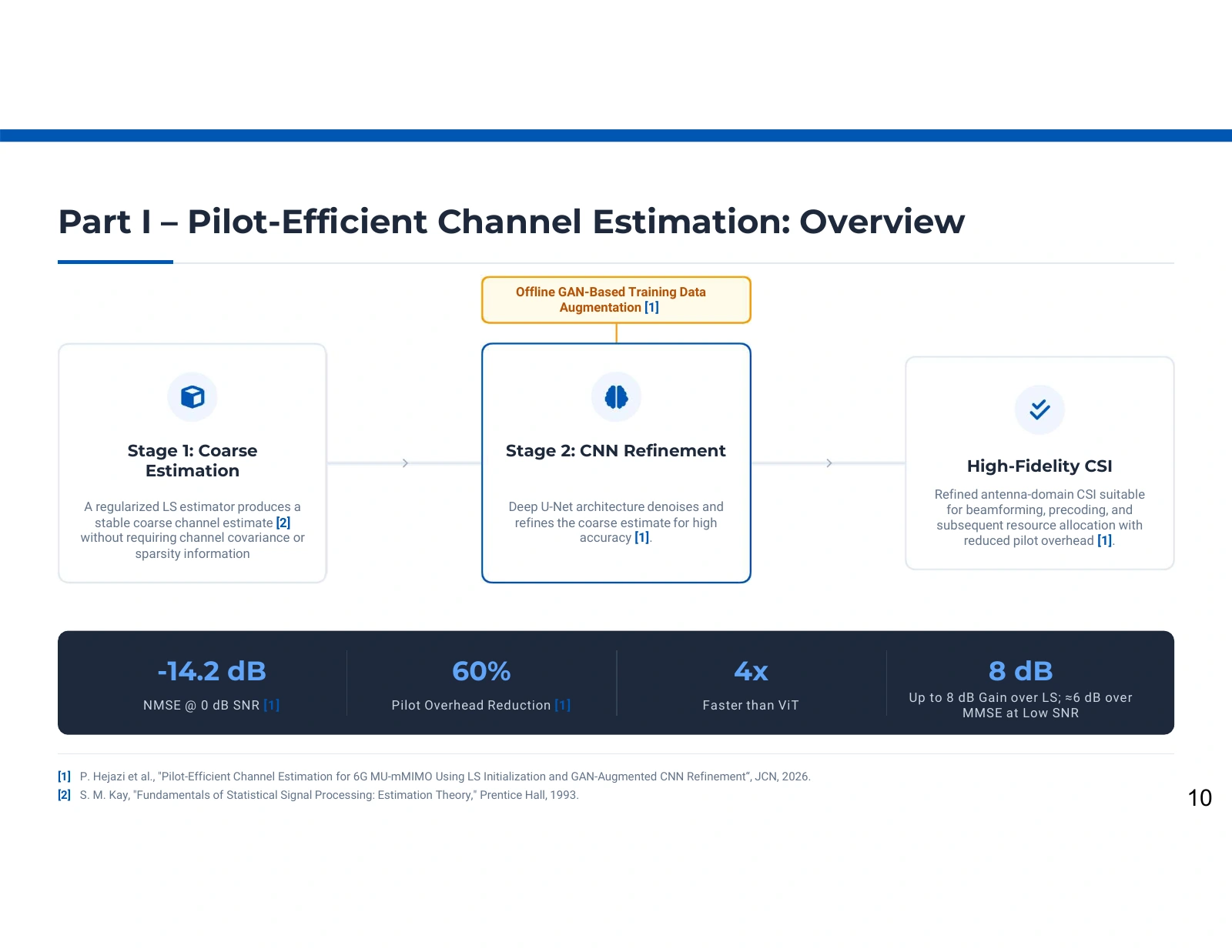
From noisy pilots to a refined channel estimate

Three connected boxes show coarse estimation, CNN refinement, and high-fidelity CSI; an orange offline GAN training box points into refinement and a dark strip lists result callouts.
From noisy pilots to a refined channel estimate. Source: Pooya Hejazi’s research presentation. Open image to inspect.

The overview separates a simple online path from an offline training branch. Least squares supplies a coarse channel estimate, the CNN refines it, and an output transformation returns the channel representation. GAN augmentation helps prepare training data; it is not an additional receiver stage for each new observation.

Read the arrows as information flow

The online input is a received pilot observation together with its known pilot matrix. The first stage produces a coarse estimate using the linear observation model. The refinement network operates on this estimate after preprocessing, rather than having to discover the entire recovery relationship from raw observations. The last box represents a channel estimate that could support subsequent communication algorithms.

Read the full explanation

Why a two-stage design is useful

The LS initialization gives the learned model a structured starting point. The CNN can focus on regularities and distortions present in the training distribution. A separate GAN branch supplies augmentation during model preparation. Keeping that branch distinct matters when interpreting cost: adversarial training and data generation are offline work, whereas the reported inference comparison concerns the deployed estimator path.

Read each callout under its own condition

The paper reports approximately −14.2 dB NMSE at 0 dB SNR and describes about an 8 dB improvement over the classical comparison. Pilot count is examined at 10 dB, while sample time is reported separately. These are not simultaneous guarantees under one universal operating point. The overview's approximate 6 dB MMSE statement, pilot percentage, and rounded timing ratio require the qualifications attached to the detailed result panels.

Technical details

  • The published channel-estimation experiment uses outdoor DeepMIMO data and selected training/testing samples.
  • The output is an estimated channel; beamforming or resource allocation benefits depend on the downstream system.

Further reading: Paper 2, Section III, Fig. 1, Algorithm 1, and Sections IV-A–IV-D. · Supplied doctoral presentation, hybrid-estimator overview.

Channel estimation

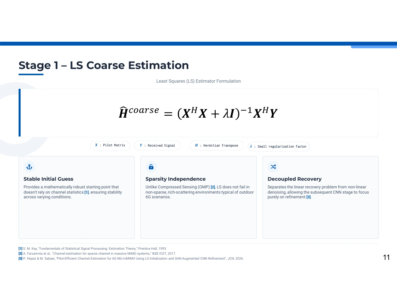
Least squares as a structured starting point

A large regularized least-squares equation sits above symbol definitions and three cards about initialization, sparsity independence, and decoupled recovery.
Least squares as a structured starting point. Source: Pooya Hejazi’s research presentation. Open image to inspect.

The regularized least-squares expression connects known pilots to the received signal and produces a coarse channel estimate. This stage supplies the refinement network with an interpretable intermediate representation. Its usefulness depends on the observation model, pilot matrix, noise, and regularization; it is not an unconditional guarantee of accurate recovery.

Read the symbols in the equation

X denotes the pilot matrix and Y the received observations. The superscript H on a matrix denotes its Hermitian, or conjugate, transpose; it is distinct from H used as the channel symbol. The identity matrix and regularization coefficient λ modify the normal-equation matrix. Together, these terms express a linear estimate from known reference signals to channel coefficients.

Read the full explanation

Why regularization and preprocessing matter

Regularization can reduce sensitivity to poorly conditioned pilot systems, at the cost of changing the estimator's bias. The diagram is a mathematical description, not an implementation instruction to form an explicit inverse. After this stage, the paper normalizes the estimate before CNN refinement. A reproducible receiver would need consistent pilot conventions, matrix dimensions, regularization settings, and transformations fitted without using unavailable target information.

What the comparison supports

Least squares does not require a sparse channel representation or a channel covariance model. That is a statement about its inputs and assumptions, not a claim that noise or rich scattering can never make recovery difficult. The proposed method learns to refine its residual errors within the training distribution. The paper's unregularized equation and regularized algorithm also differ, so the website explains the regularized conceptual path without claiming an exact code reproduction.

Technical details

  • The presentation formula and Paper 2's Algorithm 1 include regularization; the article's Eq. (7) is written without it.
  • No executable estimator, hidden normalization procedure, or unverified parameter value is supplied here.

Further reading: Paper 2, Section III-A, Eq. (7), and Algorithm 1. · Supplied doctoral presentation, coarse LS estimation.

Channel estimation

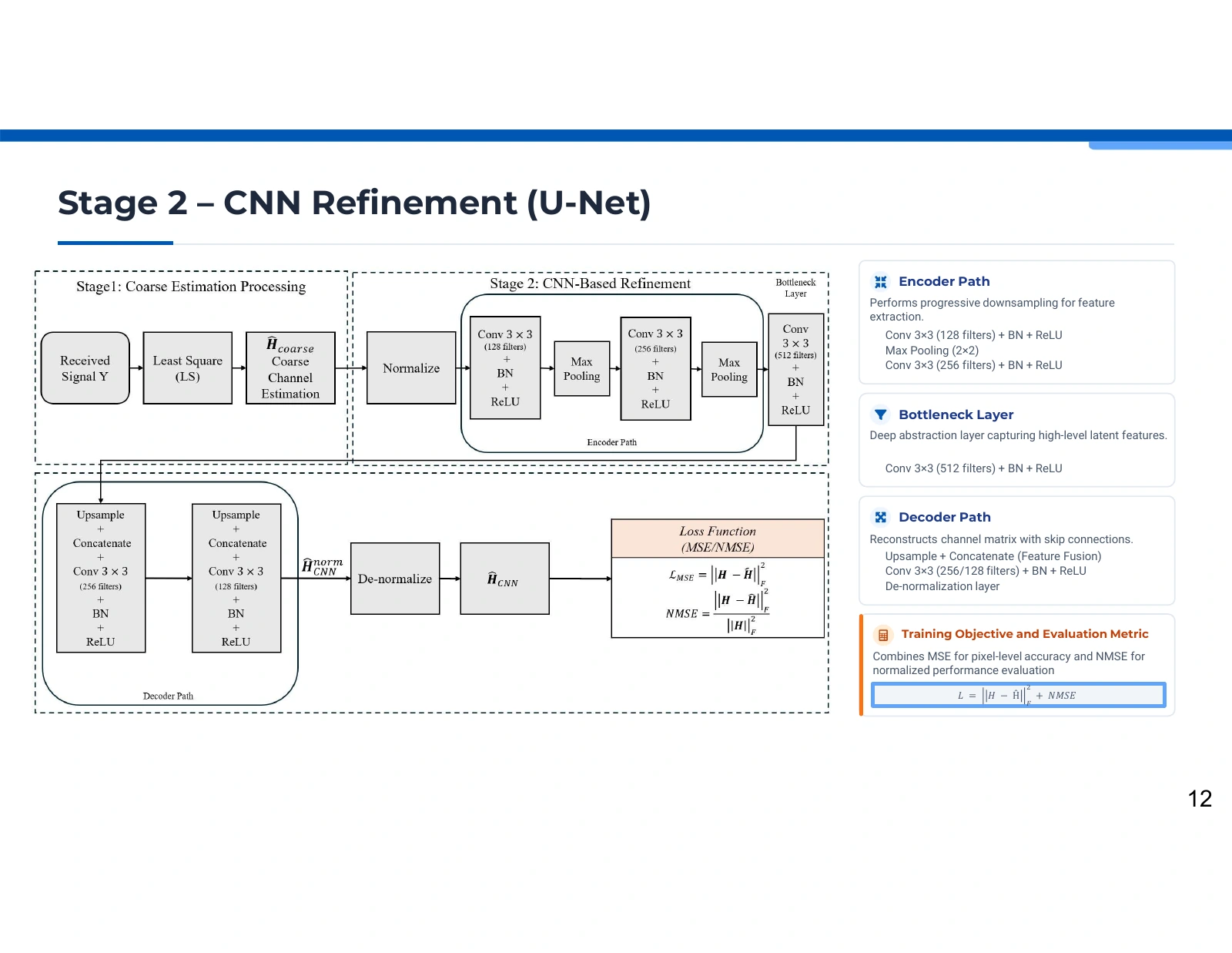
How the encoder–decoder refines channel structure

A detailed LS-to-CNN flow diagram on the left shows normalization, convolution and pooling blocks, a bottleneck, upsampling, skip connections, and de-normalization; four explanatory cards occupy the right.
How the encoder–decoder refines channel structure. Source: Pooya Hejazi’s research presentation. Open image to inspect.

The architecture diagram follows the channel estimate through normalization, feature extraction, a bottleneck, and reconstruction. Skip connections retain information across resolution changes. The network's task is channel refinement; the published training objective and evaluation metric must be distinguished from the combined-loss shorthand printed beside the diagram.

Follow the encoder and decoder

The encoder applies convolutions and progressively reduces the spatial representation to extract features. The bottleneck provides a deeper representation of those features. The decoder increases resolution and combines information carried through skip connections to reconstruct the channel representation. The image labels 3×3 convolutions and channel widths including 128, 256, and 512, illustrating the structure rather than providing a complete reproducible model specification.

Read the full explanation

Connect the architecture to the learning task

Coarse LS estimates provide the inputs, and reference channel representations supply the supervised reconstruction target. Normalization and its inverse link the network representation to the physical channel scale. The article describes convolutional blocks with batch normalization, dropout, and pooling. Training learns a mapping that reduces reconstruction error on the supplied distribution; skip connections alone do not establish robustness to every unobserved propagation environment.

Separate loss from reported accuracy

Paper 2 defines a channel-reconstruction MSE objective and reports NMSE as an evaluation measure. The presentation's adjacent formula adds MSE and NMSE, which is not the training objective specified in the article. The website preserves the diagram for explanation but uses the paper's distinction when describing learning and results. Training settings, exact tensor shapes, normalization, and synthetic input–target pairing would still need clarification for an independent reproduction.

Technical details

  • MSE is the training criterion described in Paper 2, Eq. (9); NMSE is defined for evaluation in Eq. (10).
  • GAN augmentation is part of offline data preparation and is not inside this inference diagram.

Further reading: Paper 2, Fig. 1, Section III-B, Eqs. (8)–(10), and Algorithm 1. · Supplied doctoral presentation, U-Net refinement architecture.

Channel estimation

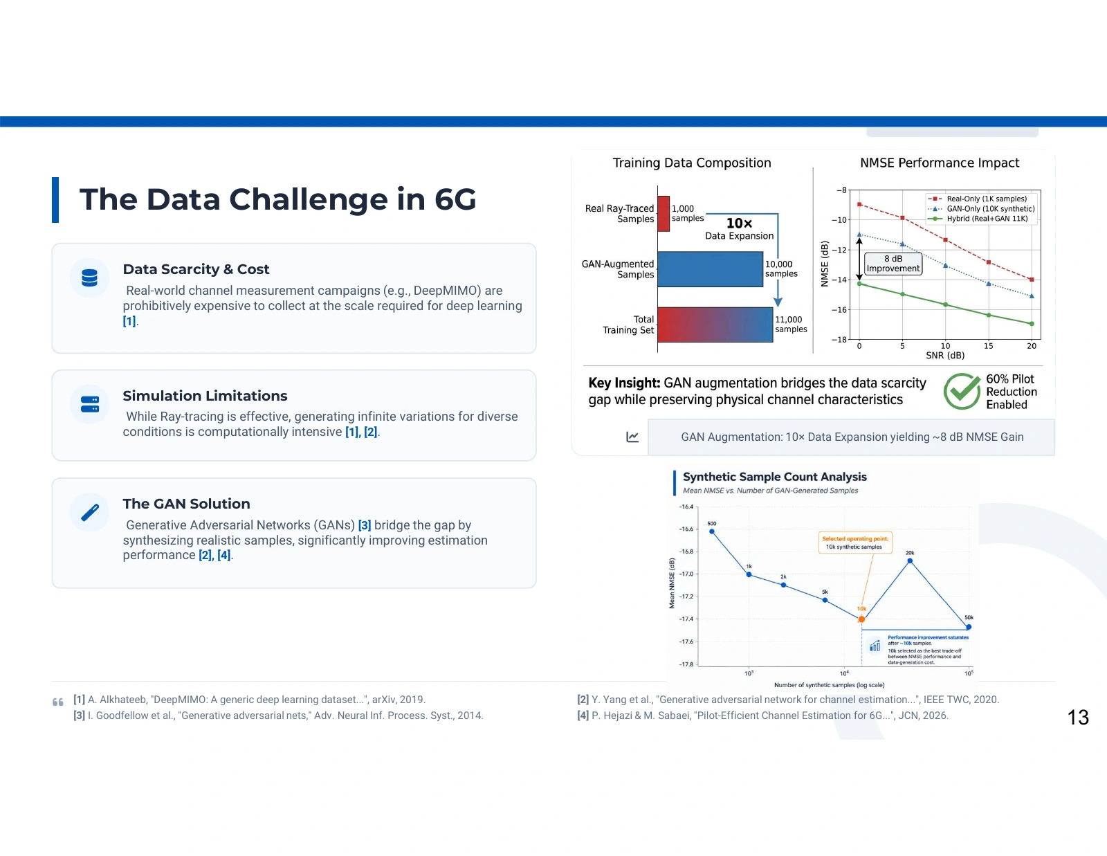
Training-data coverage and the limits of synthetic evidence

Three motivation cards on the left sit beside a 1,000/10,000/11,000-sample composition chart, an NMSE-versus-SNR illustration, and a synthetic-sample-count curve highlighting 10,000 samples.
Training-data coverage and the limits of synthetic evidence. Source: Pooya Hejazi’s research presentation. Open image to inspect.

The data panel motivates augmentation and includes sample-count, ablation, and expansion illustrations. These graphics explain the intended role of synthetic channels, but their numerical series are not established by the associated paper's published evaluation. They are preserved here with their evidence limits instead of being promoted to verified experimental tables.

Read the data categories carefully

DeepMIMO provides ray-tracing-based channel data; it should not be described here as a direct real-world measurement campaign. The image labels 1,000 original samples, 10,000 generated samples, and 11,000 total. Those are presentation labels. The printed tenfold expansion describes the generated-to-original ratio, whereas the displayed total is eleven times the original count. The article does not verify this exact sample manifest.

Read the full explanation

What augmentation is intended to accomplish

The GAN is intended to learn aspects of the training-domain channel distribution and supply additional examples for CNN preparation. More examples can be useful only if their relationship to the supervised task is valid. Distributional realism, paired targets, and independence from the evaluation set matter; a generated channel is not automatically an accurate labeled example, and more synthetic samples do not establish wider physical coverage.

Why the extra curves remain qualified

The synthetic-count sweep and real-only/GAN-only/hybrid curves do not appear as verified numerical experiments in Paper 2. Their annotations cannot establish an optimal augmentation count or isolate an 8 dB GAN contribution. The indicated gap in the illustrated ablation also does not substantiate its 8 dB callout. The published overall estimator comparison provides separate evidence and should not be confused with these unaudited presentation-only series.

Technical details

  • The article reports approximately 15% training-sample removal under its MSE filter; this differs from an augmentation ratio.
  • Synthetic samples are additional training material, not independent field measurements.

Further reading: Paper 2, Section III-C and Section IV. · Supplied doctoral presentation, data challenge and synthetic-sample illustrations.

Channel estimation

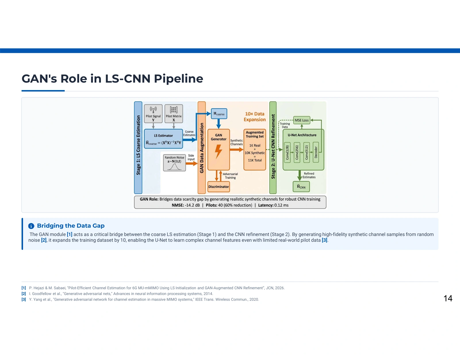
The GAN belongs to model preparation

Blue LS initialization, orange GAN augmentation, and green U-Net refinement regions show observations, pilots, random noise, generator–discriminator training, an augmented dataset, and the refined output.
The GAN belongs to model preparation. Source: Pooya Hejazi’s research presentation. Open image to inspect.

The expanded pipeline places a generator and discriminator between the LS and CNN illustrations to explain data preparation. That placement can be mistaken for an online receiver path. The published method instead uses GAN augmentation offline, then estimates a new channel through LS initialization followed by the trained CNN.

Distinguish data generation from inference

The orange region describes adversarial model preparation: a generator creates synthetic examples and a discriminator provides a training signal. Its output enters an augmented training set used to fit the refinement network. When the trained estimator processes a new pilot observation, the GAN is not called between LS and CNN. The paper's inference algorithm makes that separation clearer than the placement of the training diagram.

Read the full explanation

Understand the missing supervision detail

The LS–CNN task needs a relationship between a coarse input and a reference output. Generating a plausible channel representation alone does not specify how each synthetic input is paired with a valid target for supervised refinement. The article does not fully define that construction. The educational account therefore describes augmentation's intended role without inventing a target-generation procedure, a label, or a scaler that would create an unsupported implementation.

Interpret the labels as source annotations

The diagram repeats 1,000 original plus 10,000 synthetic samples and several performance callouts. The supplied paper does not establish this exact dataset size or a tenfold expansion experiment. Its LS expressions also differ on regularization across descriptions. These details do not invalidate the conceptual distinction between linear initialization and learned refinement, but they prevent treating this image as a complete, tested reproduction recipe.

Technical details

  • Online path: received pilots → coarse LS estimate → defined normalization → trained CNN → inverse transformation.
  • Offline path: source data and generative augmentation support training before inference.

Further reading: Paper 2, Section III-B/III-C, Eq. (11), and Algorithm 1. · Supplied doctoral presentation, GAN augmentation pipeline.

Channel estimation

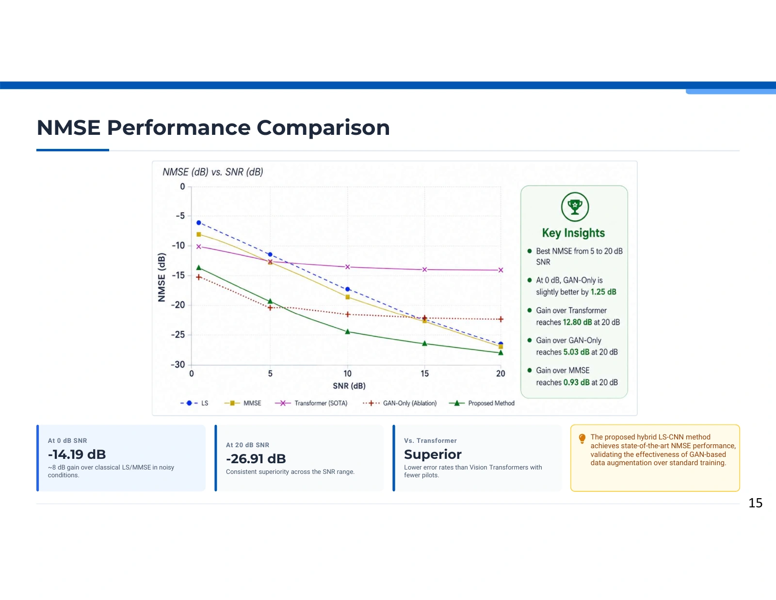
Reading estimation error across signal-to-noise conditions

A five-curve NMSE-versus-SNR chart uses blue LS circles, yellow MMSE squares, magenta Transformer crosses, red GAN-only crosses, and green proposed triangles, alongside insight and numerical callout boxes.
Reading estimation error across signal-to-noise conditions. Source: Pooya Hejazi’s research presentation. Open image to inspect.

The NMSE chart compares the proposed estimator with classical, Transformer, and GAN-only curves across increasing SNR. More negative NMSE indicates lower relative channel error. The plot supports a discussion of how comparisons change with noise, while conflicts between its annotations and the published figure prevent treating every displayed value as a verified result.

Read one operating condition at a time

The horizontal axis gives SNR; the vertical axis gives NMSE in dB. Comparing methods at the same SNR asks how accurately they estimate channels under a common noise condition. Moving along one curve asks how that estimator behaves as the signal becomes stronger relative to noise. A difference in dB describes a ratio of normalized errors, not an equal number of percentage points.

Read the full explanation

Use the published low-SNR statement

The associated paper reports approximately −14.2 dB for the proposed framework at 0 dB SNR and describes about an 8 dB improvement over its classical comparison. The presentation prints −14.19 dB and a separate −26.91 dB high-SNR callout. These more precise labels should not imply additional measurement precision, confidence intervals, or an independently reproduced sweep. Training and testing also use the source's quality-based sample selection.

Keep internal disagreements visible

The presentation's plotted high-SNR endpoint does not agree with its own −26.91 dB card, and the curve differs from the article's figure. Its own insight box also acknowledges GAN-only performing better at the lowest SNR, so “consistent superiority” is too broad even within this image. The other pairwise gain annotations remain source annotations; they are not used to create a new numerical dataset or establish a general state-of-the-art ranking.

Technical details

  • This is channel-reconstruction NMSE, not bit-error rate or decoding reliability.
  • Paper 2's reported evaluation is over 0–20 dB in its outdoor DeepMIMO setup.

Further reading: Paper 2, Section IV-A, Fig. 3, and Section III-C. · Supplied doctoral presentation, NMSE comparison.

Channel estimation

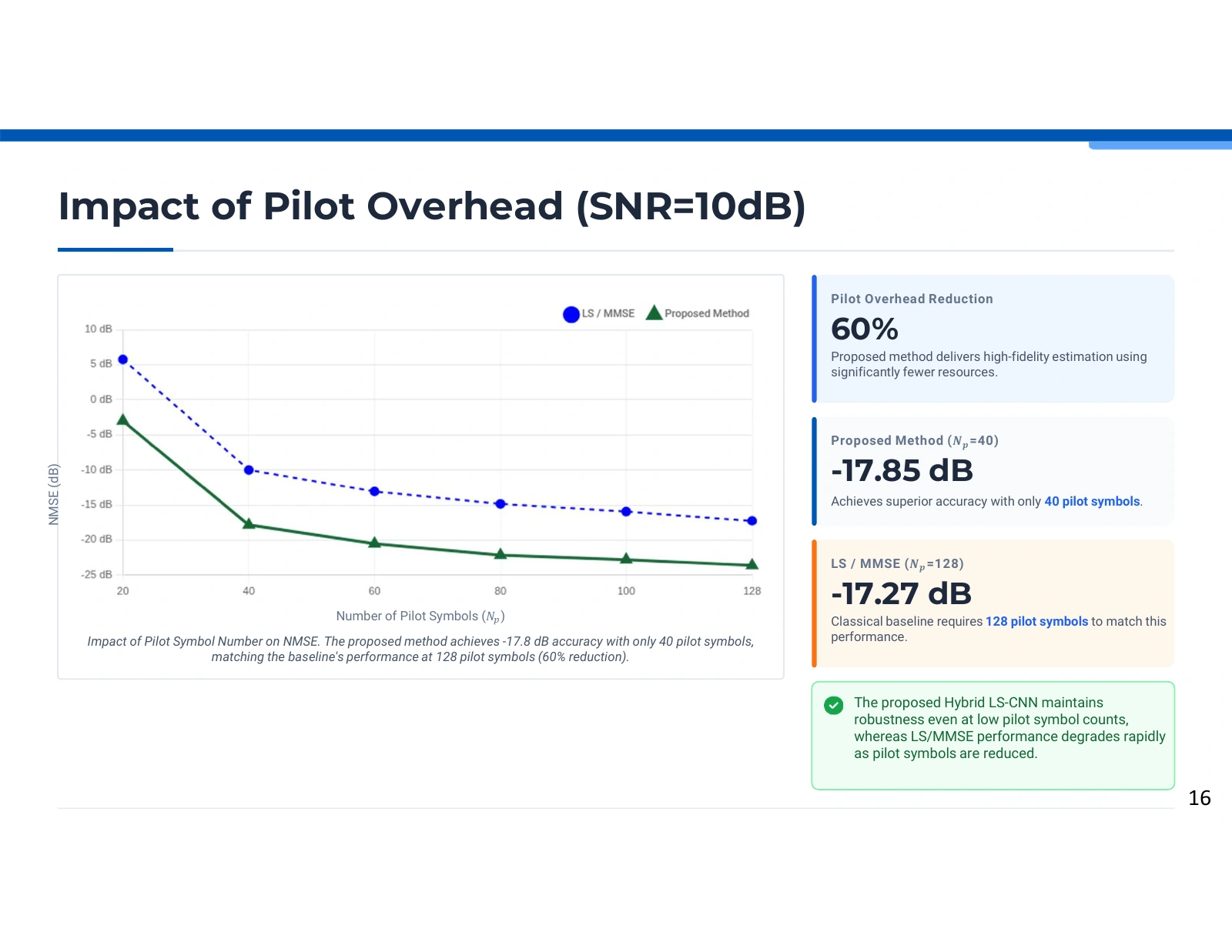
What fewer pilots mean at a fixed noise level

A two-curve graph plots NMSE against pilot count, using blue baseline circles and green proposed triangles; adjacent cards highlight 40 pilots, 128 pilots, and a 60% reduction claim.
What fewer pilots mean at a fixed noise level. Source: Pooya Hejazi’s research presentation. Open image to inspect.

The pilot-count plot fixes SNR at 10 dB and varies the number of reference symbols. It illustrates the study's central resource trade-off: learned refinement can improve the reported error at a given pilot budget. The highlighted 40-versus-128 comparison is useful, but its error labels and reduction percentage are inconsistent across the sources.

Compare matched horizontal positions first

At any one pilot count, the two curves compare reported estimation errors under the fixed 10 dB SNR condition. Following either curve shows how its error changes as more reference symbols are provided. This differs from the SNR sweep: the noise condition is held fixed while the measurement budget changes. A smaller pilot budget may leave more transmission resources for payload, subject to the complete frame design.

Read the full explanation

What the source actually highlights

The presentation labels the proposed result at 40 pilots as −17.85 dB and the baseline at 128 pilots as −17.27 dB. The paper's figure caption instead rounds the former to −17.8 dB, while its nearby prose says approximately −16 dB at 40 pilots. These are source-specific statements, not measurements independently reconstructed here. The defensible narrative is that the study reports useful refinement with fewer pilots; exact equivalence remains unresolved.

Keep the arithmetic and experiment separate

Reducing a count from 128 to 40 corresponds arithmetically to 68.75%, so the printed 60% does not follow from those counts. That arithmetic check does not resolve the mismatched error descriptions or validate an optimal pilot policy. The source's stated search interval also does not fully match its plotted counts. The website preserves the original curve and identifies these differences rather than inventing a corrected experimental result.

Technical details

  • The proposed and baseline values use different pilot counts in the highlighted comparison.
  • A pilot-count reduction is not automatically an identical percentage increase in end-to-end data throughput.

Further reading: Paper 2, Section IV-C and Fig. 5; pilot-search description in Section III-C. · Supplied doctoral presentation, pilot-count comparison at 10 dB.

Channel estimation

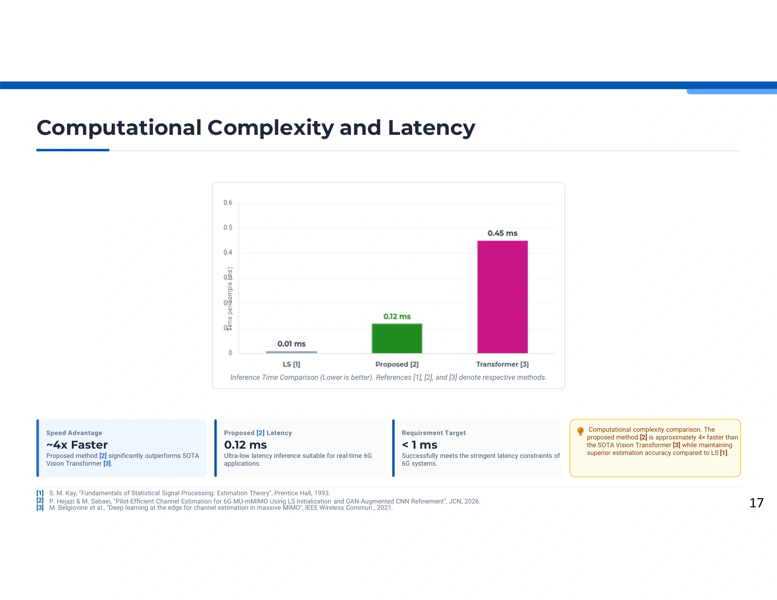
Inference time is one part of computational cost

Three vertical bars show LS at 0.01 ms, the proposed method at 0.12 ms, and the Transformer at 0.45 ms, above cards about speed and a sub-millisecond target.
Inference time is one part of computational cost. Source: Pooya Hejazi’s research presentation. Open image to inspect.

The bar chart reports time per sample for three estimators: LS, the proposed model, and a Transformer baseline. It shows the study's accuracy–runtime trade-off, with learned refinement costing more than LS but less than the configured Transformer. The timing values describe this comparison rather than a hardware-independent latency guarantee.

Read the measured quantity precisely

The vertical axis is time per sample in milliseconds. The source reports 0.01 ms for LS, 0.12 ms for the proposed estimator, and 0.45 ms for the Transformer comparison. The ratio between the latter two values is 3.75, summarized as approximately fourfold in the presentation. LS is still the fastest reported option; the learned stage is motivated by its estimation behavior, not by beating LS in raw sample time.

Read the full explanation

Distinguish parameter count from latency

The article describes approximately 8.35 million trainable parameters for the proposed U-Net and approximately 0.34 million for its Transformer baseline. A larger parameter count can coexist with a shorter measured runtime because computation structure and execution conditions matter. This result therefore does not establish that the CNN is the smaller model, nor that every CNN will run faster than every Transformer.

Avoid extending the bars to system guarantees

The paper does not specify enough hardware, batching, timing repetition, or implementation context for a portable latency benchmark. Time spent collecting pilots, moving data, scheduling users, or decoding payload is also different from estimator sample time. A value below one millisecond in this plot is not proof that an entire communication service meets every latency requirement. Deployment conclusions need measurements for the complete intended workload.

Technical details

  • Reported values are from the study; the website has not rerun a runtime benchmark.
  • The generative augmentation process is offline and should not be counted as a per-observation GAN call.

Further reading: Paper 2, Transformer baseline description, Section IV-D, and Fig. 6. · Supplied doctoral presentation, inference-time comparison.

Channel estimation

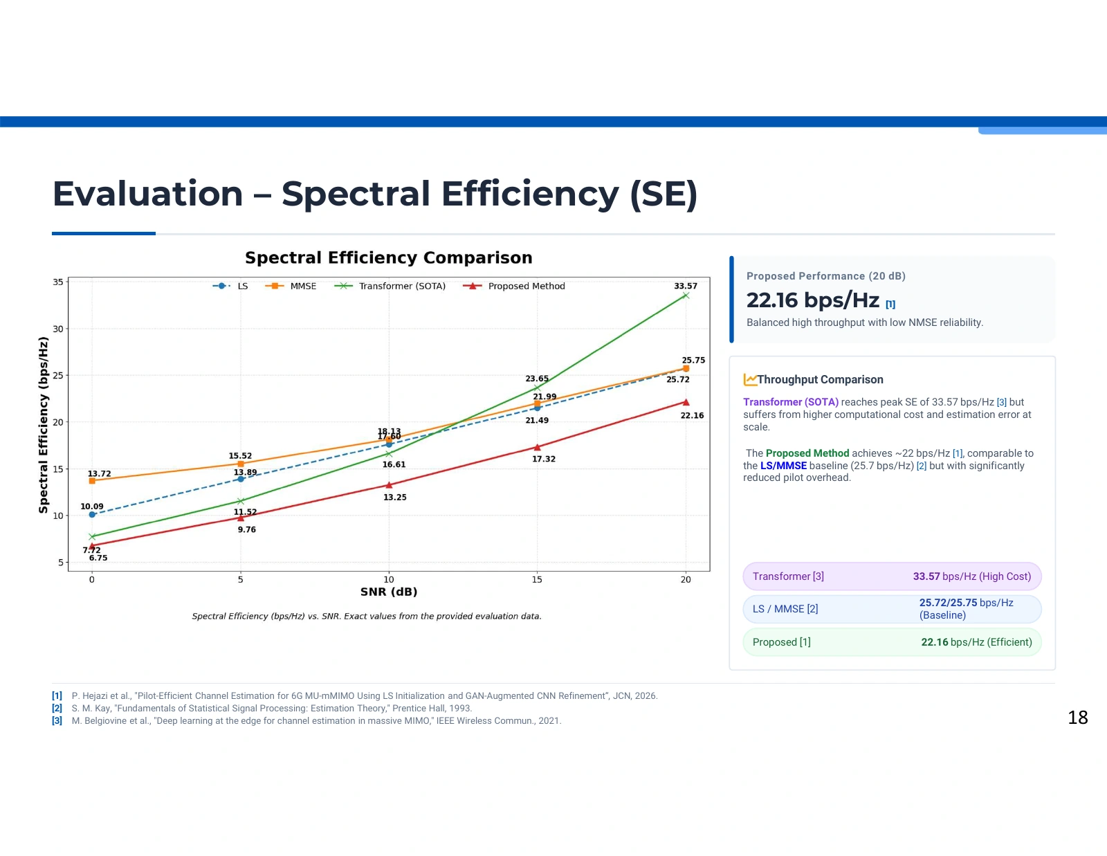
Estimation error and spectral efficiency answer different questions

A four-curve spectral-efficiency chart labels values from 0 to 20 dB SNR; blue LS, orange MMSE, green Transformer, and red proposed curves sit beside endpoint comparison cards.
Estimation error and spectral efficiency answer different questions. Source: Pooya Hejazi’s research presentation. Open image to inspect.

The spectral-efficiency plot provides a second perspective on the estimator comparison. It reports increasing modeled rates with SNR, while the proposed method's curve remains below the displayed alternatives. This matters: a favorable NMSE result should not be described as universal superiority in throughput, reliability, or every downstream communication metric.

Read rate separately from reconstruction error

The vertical axis is spectral efficiency in bit/s/Hz, while the horizontal axis is SNR. The image labels the proposed endpoint at 20 dB as 22.16 bit/s/Hz, compared with 25.72 for LS, 25.75 for MMSE, and 33.57 for the Transformer. These are explicit presentation annotations. They describe a rate-related model output, whereas NMSE measures the discrepancy between estimated and reference channels.

Read the full explanation

Recognize the trade-off shown by the curves

The proposed curve is lower than the alternatives displayed in this image, so it cannot support a claim that the estimator has the highest spectral efficiency in this comparison. Its research argument also considers pilot use, error, and inference cost. Combining those into an end-to-end conclusion would require compatible pilot accounting, receiver processing, and rate definitions, rather than selecting the most favorable metric from different experiments.

Keep precision and provenance visible

The article summarizes the proposed result as approximately 23 bit/s/Hz at 20 dB, while this presentation gives 22.16. The website does not silently replace one with the other or digitize new values from curve pixels. Neither the plot nor a lower NMSE establishes a measured bit-error rate, decoding reliability, or live-network throughput. The baseline reference labels likewise do not independently establish the precise implementation used to produce every curve.

Technical details

  • At 20 dB, the presentation labels are: proposed 22.16; LS 25.72; MMSE 25.75; Transformer 33.57 bit/s/Hz.
  • The article's approximate prose value and the presentation's more precise label are retained as distinct source statements.

Further reading: Paper 2, Section IV-B and Fig. 4. · Supplied doctoral presentation, spectral-efficiency comparison.

Channel estimation

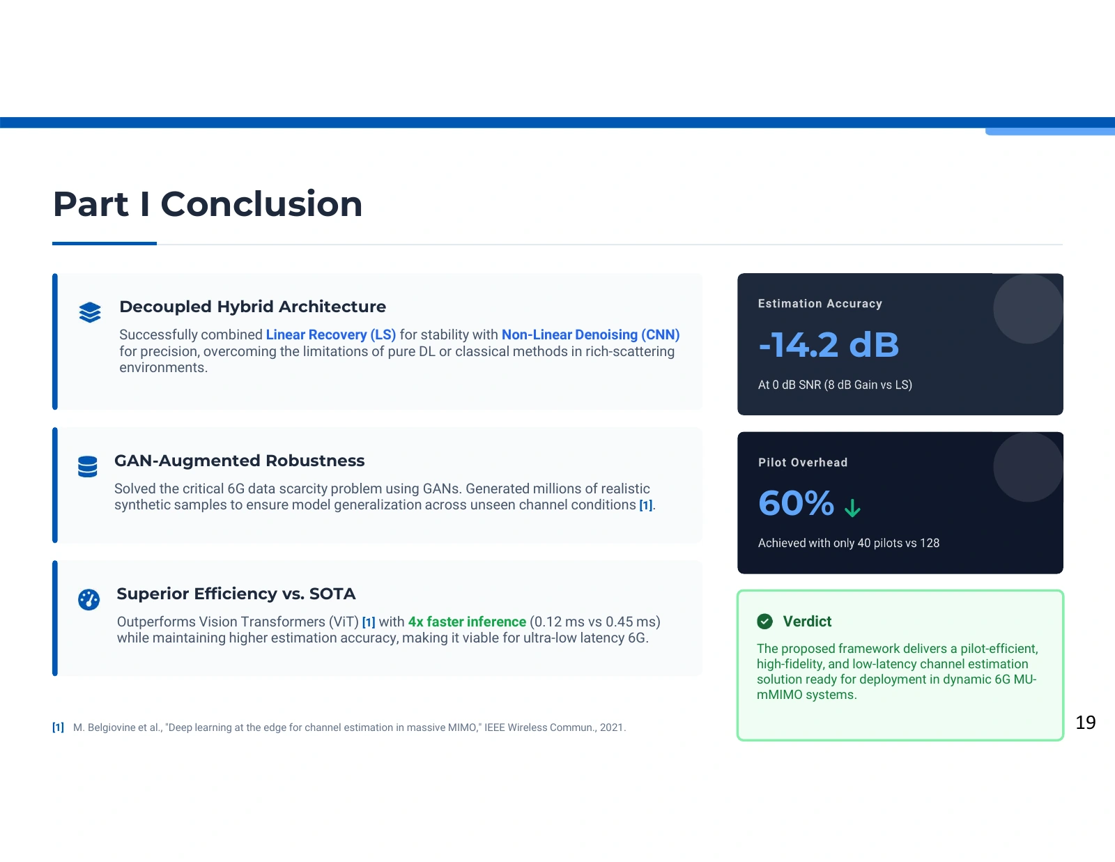
What the channel-estimation study establishes

Three conclusion cards describe the hybrid architecture, GAN augmentation, and runtime; dark callouts show −14.2 dB and 60%, with a green deployment verdict box.
What the channel-estimation study establishes. Source: Pooya Hejazi’s research presentation. Open image to inspect.

The conclusion brings the hybrid architecture, augmentation idea, and reported efficiency results together. Its strongest supported outcome is a conditional estimation result in the paper's selected DeepMIMO evaluation. Statements that data scarcity is solved, millions of generated samples ensure generalization, or the method is deployment-ready go beyond the supplied evidence.

The architecture contribution is clear

The method separates linear recovery from learned refinement. LS produces an interpretable starting estimate, and the CNN learns corrections from the available channel data. GAN augmentation is used in training rather than adding an online receiver stage. This organization is the central design contribution and can be understood without publishing an implementation or treating an ambiguous script as a faithful reproduction.

Read the full explanation

The results remain tied to their experiments

The paper reports approximately −14.2 dB NMSE at 0 dB SNR, a smaller highlighted pilot budget, and 0.12 ms time per sample in its runtime comparison. These results answer different questions under selected conditions. Sample filtering, conflicting pilot annotations, and missing timing context affect interpretation. The accompanying spectral-efficiency comparison also illustrates why the result should be described as a trade-off rather than superiority on every measure.

What would strengthen the next stage

Generalization should be evaluated on genuinely separate sites, propagation conditions, and mobility regimes, with clearly documented data splits and preprocessing. Receiver-level error measurements and repeated timing on identified hardware would support deployment claims. An audited augmentation manifest and an explicit synthetic input–target construction would clarify the training contribution. These are validation directions, not additional experiments or achievements claimed by the website.

Technical details

  • The source does not verify the conclusion's claim of millions of generated training samples.
  • The final article identifies further channel scenarios and refinement approaches as future work.

Further reading: Paper 2, Sections III-C, IV, and V. · Supplied doctoral presentation, channel-estimation conclusion.

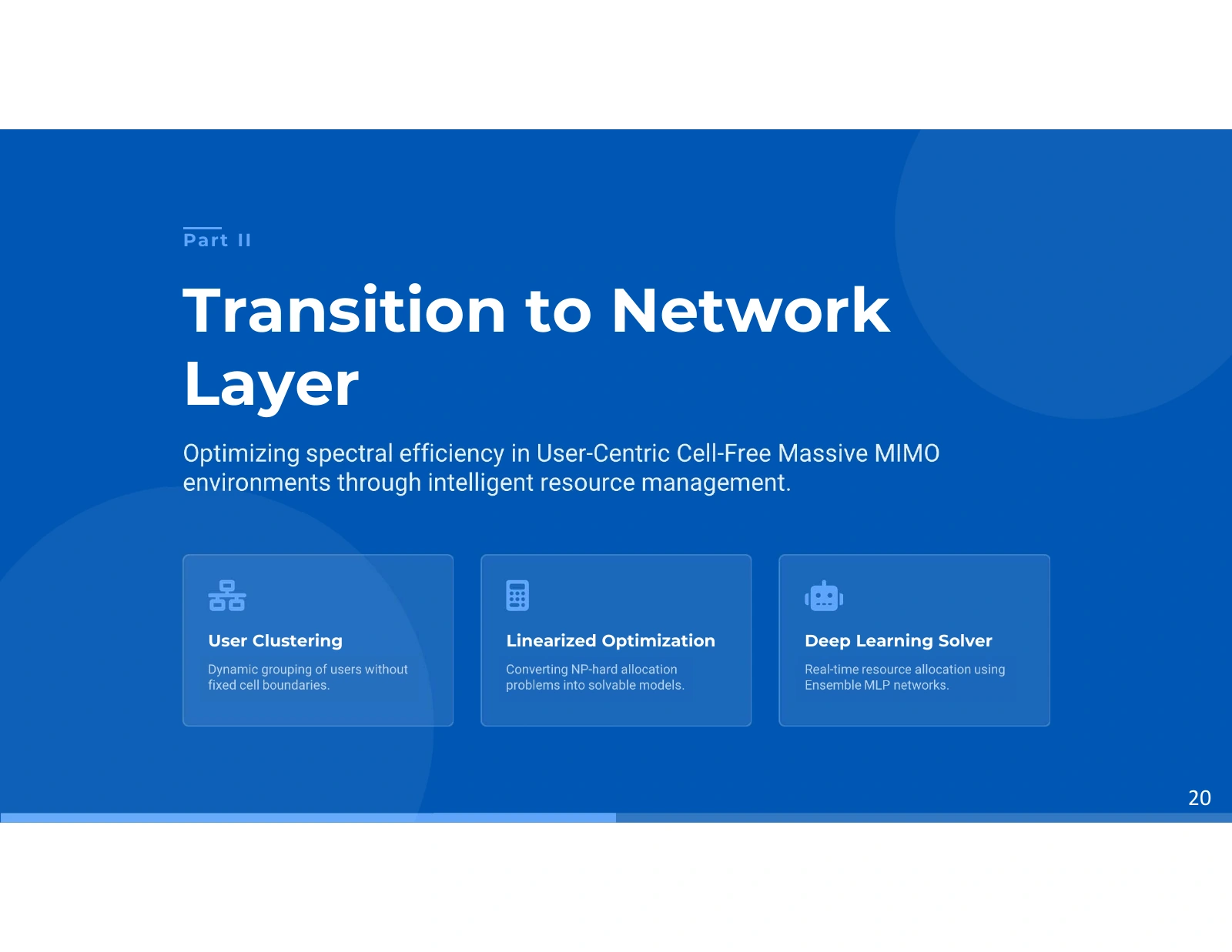
User clustering

From channel information to network decisions

A blue transition panel presents three translucent cards for user clustering, linearized optimization, and a deep-learning solver, beneath a large network-layer heading.
From channel information to network decisions. Source: Pooya Hejazi’s research presentation. Open image to inspect.

The transition changes the object of prediction: the first study estimates channel coefficients, while the second proposes user groups and resource assignments. Both use physical structure to guide learning, but they have different inputs, outputs, objectives, and tests. Their connection is a research direction rather than a demonstrated combined pipeline.

A different decision level

A channel estimate describes propagation. An allocation decision selects how modeled users and resources should interact. The clustering study uses channel-dependent information to reason about spectral efficiency and feasible assignments.

Read the full explanation

The offline-to-online strategy

An optimization formulation supplies labeled examples for training. A neural model then predicts assignments from new channel features. This parallels the estimation study's use of structured preparation, but the predictor and the meaning of its output are different.

What the transition implies

The following material explains the network model, objective, constraints, linearization, and learned predictor. It does not establish that the preceding LS–CNN estimator was inserted into this allocation experiment. Evaluating error propagation between the two methods would be a separate integration study.

Technical details

  • The clustering paper's reported metrics and assumptions apply to its own experimental setup.

Further reading: Paper 1, Introduction and Sections II–IV. · Paper 2, Section III. · Supplied doctoral presentation, transition to resource allocation.

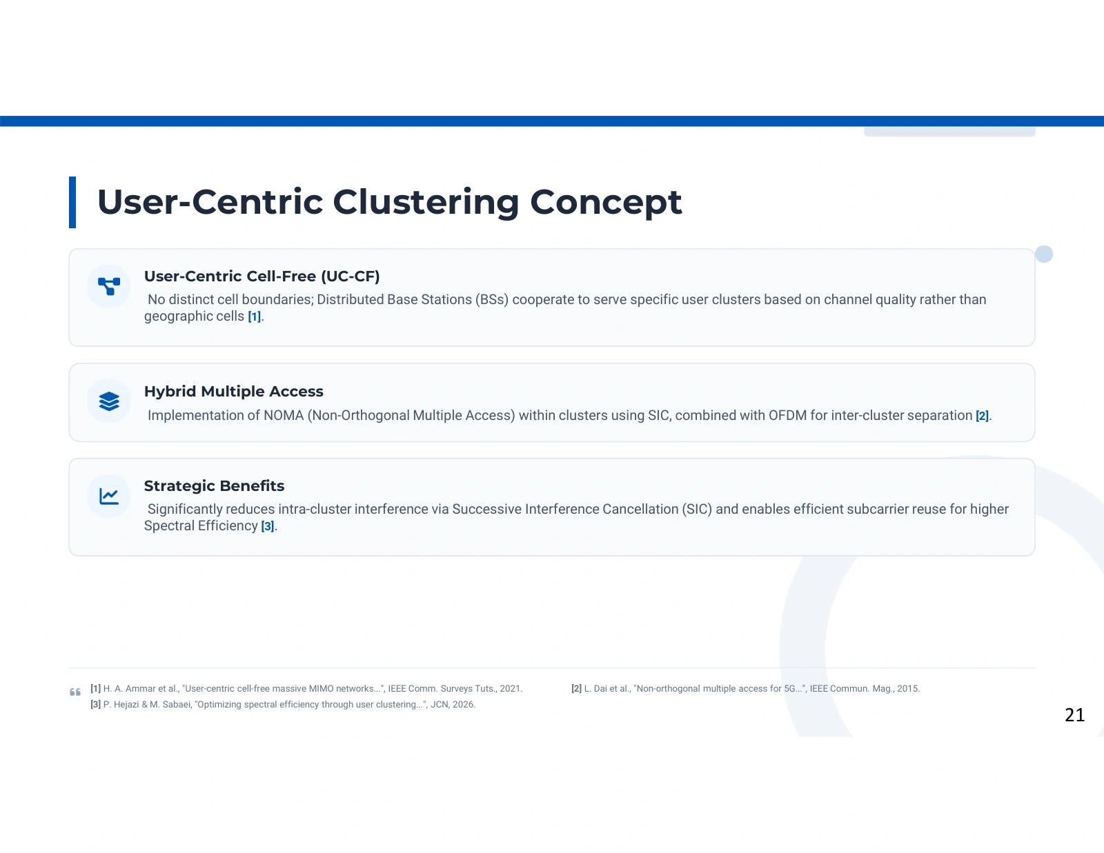
User clustering

User-centric grouping and shared radio resources

Three broad text cards define user-centric cell-free operation, the combination of NOMA and OFDM, and intended interference-management benefits.
User-centric grouping and shared radio resources. Source: Pooya Hejazi’s research presentation. Open image to inspect.

The concept panel explains a user-centric alternative to fixed cell boundaries. Distributed base stations and radio resources are coordinated around user groups, with NOMA and SIC inside the modeled clusters and OFDM resources used for separation. The benefits depend on the channel, receiver assumptions, and allocation rules.

What user-centric means in this study

The allocation model is organized around groups of users and the resources serving those groups. Channel-dependent relationships matter rather than only a fixed geographic cell partition. The paper defines user membership and base-station/subcarrier assignment variables to make those relationships explicit. The objective is to choose useful combinations under the stated network constraints, not to assume that removing cell boundaries removes every resource limitation.

Read the full explanation

How the multiple-access components interact

NOMA allows modeled users within a cluster to share a resource. SIC is the receiver mechanism assumed to separate their contributions through successive decoding and cancellation. OFDM provides subcarriers that can be assigned across clusters and base stations. These components create an allocation trade-off: grouping and reuse can increase resource utilization, but the resulting interference and decoding conditions influence the rates that are actually achievable.

Why the assumptions remain important

The paper considers quasi-static or slowly changing topology and favorable propagation conditions. Its rate and assignment results inherit those assumptions. Imperfect cancellation, channel-estimation errors, synchronization, and implementation constraints would need separate assessment before extrapolating to a deployed distributed system. The concept diagram motivates the optimization model; it is not a measurement proving interference-free communication or a universal improvement over every fixed-cell configuration.

Technical details

  • User membership and serving-resource assignment are separate binary decisions in Paper 1.
  • NOMA and SIC here describe the modeled receiver and resource-sharing assumptions.

Further reading: Paper 1, Section II and Section II-A, including Fig. 2. · Supplied doctoral presentation, user-centric clustering concept.

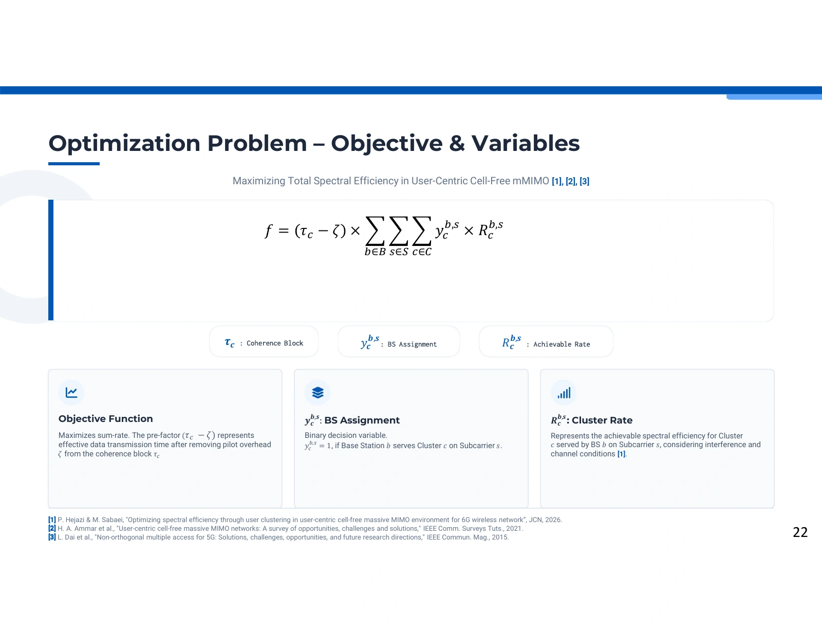
User clustering

An objective that couples useful transmission time and rate

A large equation multiplies the remaining coherence-block term by a triple sum of binary assignments and cluster rates; symbol chips and three explanation cards sit below it.
An objective that couples useful transmission time and rate. Source: Pooya Hejazi’s research presentation. Open image to inspect.

The objective sums rates over selected base-station, subcarrier, and cluster assignments, weighted by the coherence-block resources remaining after pilots. It expresses why grouping cannot be judged by channel strength alone: a decision changes both the serving configuration and the resource costs included in the model.

Read the decision variable and rate together

The binary variable y identifies whether a base station serves a cluster on a particular subcarrier. Multiplying it by the corresponding cluster-rate term includes the rate only when that assignment is selected. Summation then aggregates the selected combinations. User-membership variables enter the underlying channel and rate model even though the compact objective shown here emphasizes the serving-resource variable.

Read the full explanation

Why pilot overhead appears in the objective

The factor τc − ζ represents the block resources remaining after the modeled pilot requirement. In the paper, τc is expressed in symbols and ζ is associated with a maximum pilot length and cluster size. The design therefore links allocation choices to the useful portion of the coherence block. The expression retains the source's convention; interpreting it as a normalized spectral-efficiency value requires specifying the rate and block normalization.

The objective is only part of the problem

Maximizing this expression without membership, serving-resource, cluster-size, connectivity, and receiver constraints would solve a different task. The following formulation introduces those conditions and then approximates nonlinear components for label generation. Neither a large objective value nor a close neural prediction proves feasibility automatically. The source's pilot definition and some constraint indices are ambiguous, so this explanatory equation is not presented as validated executable optimization code.

Technical details

  • Paper 1 defines the original objective in Eq. (1), the block size in Eq. (2), and the pilot-length expression in Eq. (3).
  • A symbol-count prefactor should not silently be treated as a dimensionless per-symbol efficiency factor.

Further reading: Paper 1, Section II-A, Eqs. (1)–(11); Section II-B for the approximation. · Supplied doctoral presentation, objective and variables.

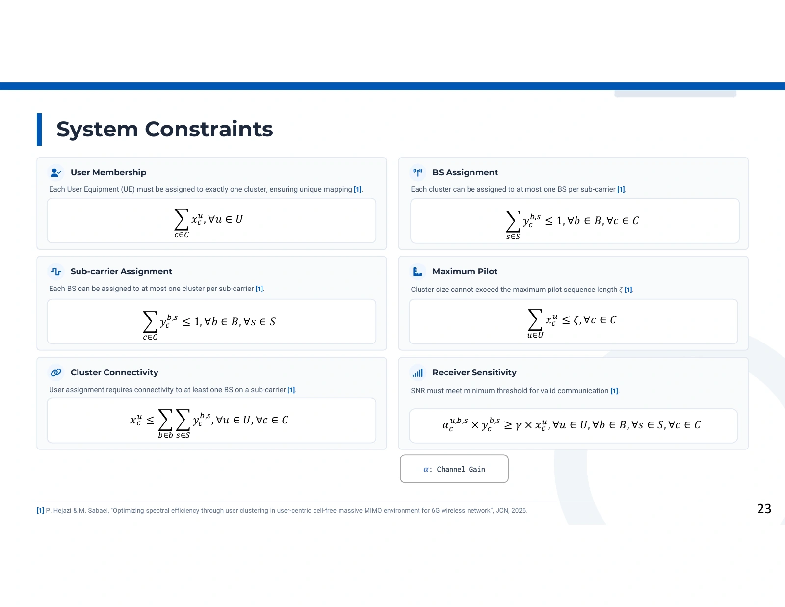
User clustering

The rules behind a feasible allocation

Six constraint panels describe user membership, base-station assignment, subcarrier assignment, maximum pilot length, cluster connectivity and receiver sensitivity, with their associated expressions.
The rules behind a feasible allocation. Source: Pooya Hejazi’s research presentation. Open image to inspect.

Membership, connectivity, resource sharing and pilot limits define which assignments the optimizer may consider. Each condition addresses a different physical or scheduling requirement.

Membership and connectivity

A user belongs to one cluster, so membership is an equality rather than an invitation to select any number of groups. Connectivity then links that membership decision to an available base-station/subcarrier assignment. Without this relationship, an optimizer could assign users to a cluster that has no serving resources and still count an apparent benefit.

Read the full explanation

Shared resources and pilot limits

The assignment variables describe a cluster, base station and subcarrier together. Summing over a particular index determines which combinations are restricted, so changing an index changes the scheduling rule. The pilot-related condition bounds cluster size by the available sequence length. It connects the network allocation problem to the training resources needed to estimate channels.

Feasibility as a separate question

The receiver-sensitivity condition introduces a minimum acceptable link quality. These constraints define the feasible set before the objective selects a preferred assignment. When a neural model later predicts the decision variables, a low classification loss alone does not prove that every constraint holds. A deployment-oriented interpretation therefore distinguishes label accuracy from explicit constraint checking.

Technical details

  • Read the membership condition as one cluster per user, consistent with Paper 1 Eq. (6).
  • Interpret each assignment inequality using its summation indices, not only its short panel label.

Further reading: Paper 1, Section II.A, PDF pp. 4-5, Eqs. (6)-(11). · Supplied presentation, System Constraints.

User clustering

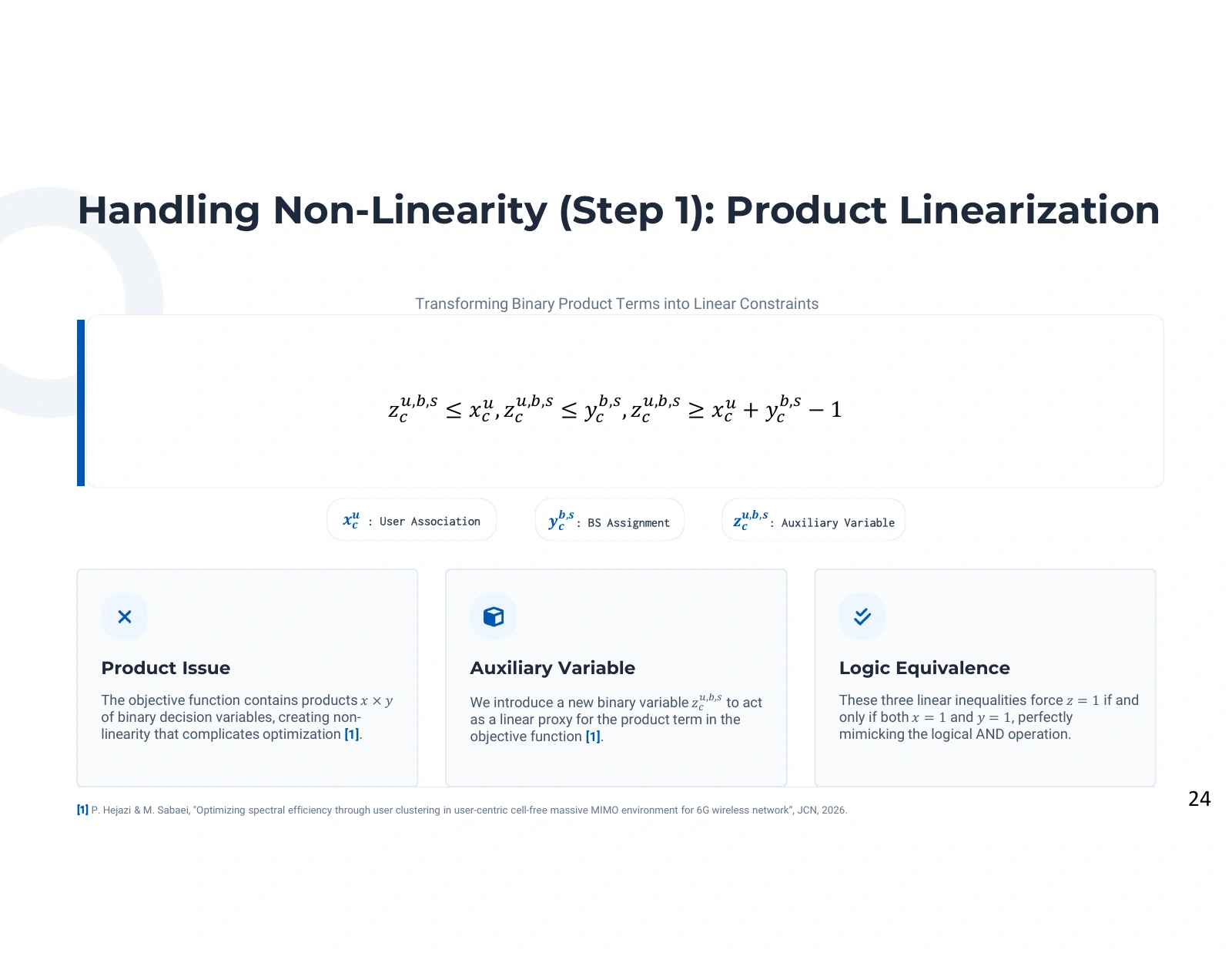
Representing joint decisions with auxiliary variables

A product-linearization explanation introduces z for the product of user membership x and base-station assignment y, with the inequalities z no greater than x or y and z at least x plus y minus one.
Representing joint decisions with auxiliary variables. Source: Pooya Hejazi’s research presentation. Open image to inspect.

An auxiliary variable represents the product of two binary assignment decisions. Three linear inequalities preserve the logical relationship without multiplying the decisions directly.

Why a product appears

A user's contribution can depend on two choices being active together: membership in a cluster and assignment of resources to that cluster. Multiplying the associated binary variables expresses that conjunction. The resulting interaction is nonlinear in the decision variables, which complicates an otherwise linear optimization formulation.

Read the full explanation

What the auxiliary variable means

The construction introduces z to carry the joint decision. If either x or y is zero, the upper inequalities force z to zero. If both are one, the lower inequality forces z to one. For binary decisions, this is an exact representation of the product. It preserves the meaning of the original logical interaction rather than approximating its value.

What linearization does not guarantee

Removing a product makes the formulation compatible with mixed-integer linear optimization machinery, but the binary search space remains. The transformation does not turn the overall combinatorial problem into a polynomial-time problem. Its role in this research is to make offline label generation more manageable while preserving the relevant assignment coupling.

Technical details

  • The exact binary construction is z ≤ x, z ≤ y and z ≥ x + y − 1, together with the declared variable domains.
  • If the binary domains are later relaxed, these inequalities describe the product's linear relaxation; z is no longer automatically equal to xy for fractional x and y.

Further reading: Paper 1, Section II.B, PDF pp. 5-6, auxiliary-variable constraints. · Supplied presentation, Product Linearization.

User clustering

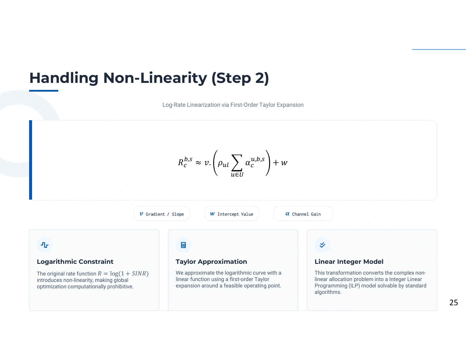
Approximating the logarithmic rate

The logarithmic rate is represented by a first-order expression using a slope v and intercept w, followed by explanations of the logarithmic constraint, Taylor approximation and integer linear model.
Approximating the logarithmic rate. Source: Pooya Hejazi’s research presentation. Open image to inspect.

A first-order Taylor expression replaces a curved rate relationship with a local linear approximation. This simplifies optimization while introducing an approximation boundary.

The source of nonlinearity

The rate expression depends on a logarithm of a signal-quality quantity. Increasing channel gain improves the modeled rate, but the improvement is not linear. This diminishing-return relationship matters because an optimizer choosing among links should not assume that doubling a signal-quality term necessarily doubles the corresponding achievable rate.

Read the full explanation

The local linear model

A first-order expansion uses the rate's value and slope at a chosen operating point. The displayed coefficients v and w summarize the slope and intercept. Once fixed, they allow the objective to use linear coefficients. Unlike the binary-product substitution, this step approximates the numerical objective and is most informative near the operating point used to construct it.

Interpreting the resulting labels

Assignments generated by the linearized model optimize that model under its specified constraints. Their quality for the original nonlinear rate should be assessed by evaluating the original expression or by a justified approximation analysis. The presentation explains the modeling route to training labels; it does not establish that every resulting assignment is globally optimal for the unapproximated wireless system.

Technical details

  • The operating point and approximation range affect the accuracy of a Taylor model.
  • A linear objective with integer decisions remains an integer optimization problem; linearity of expressions does not remove combinatorial complexity.

Further reading: Paper 1, Section II.B, PDF pp. 5-6, rate linearization. · Supplied presentation, Handling Non-Linearity.

User clustering

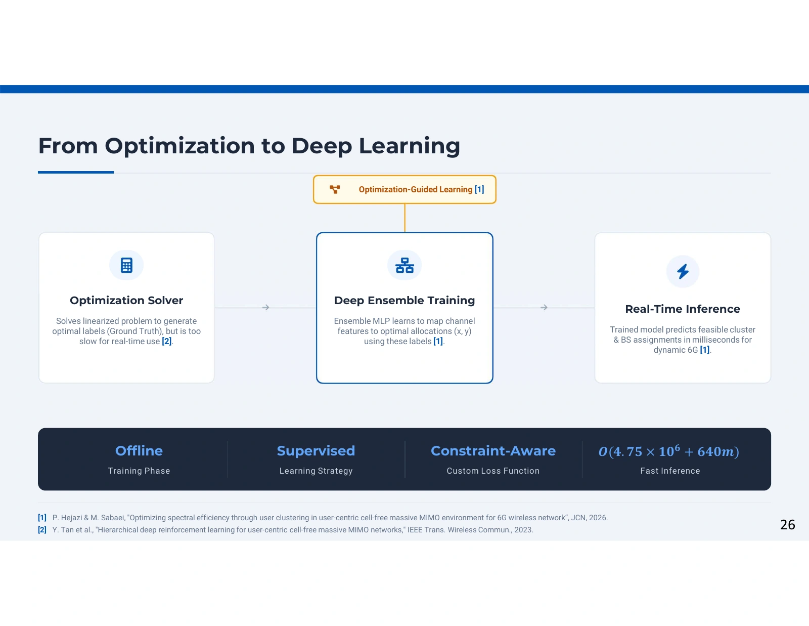
Learning from optimization-generated assignments

Three connected stages show an optimization solver, deep ensemble training and fast inference, with notes on offline training, supervised learning and a constraint-aware loss.
Learning from optimization-generated assignments. Source: Pooya Hejazi’s research presentation. Open image to inspect.

The framework spends computation offline to generate allocation labels, then trains a neural predictor to approximate those decisions for new modeled network instances.

Offline labels

The optimization model maps a network instance to cluster and resource assignments. Its inputs describe the modeled channel and geometry, while its constraints specify admissible choices. Solving many such instances produces feature-label pairs. This stage can be expensive because it is part of dataset construction rather than the immediate response to every live scheduling request.

Read the full explanation

Supervised approximation

The neural model learns a mapping from the instance features to the assignment variables. The training objective combines agreement with solver-generated labels and penalties associated with allocation constraints. The predictor therefore receives guidance about both the desired outputs and the structure of the underlying scheduling problem, although penalties do not constitute an exact feasibility certificate.

Online use and its limits

After training, a forward pass replaces a fresh optimization solve for the evaluated setting. The resulting speed advantage concerns the online prediction stage and excludes the earlier costs of generating labels and fitting the model. Generalization depends on how closely a new topology and channel distribution resemble the training and test instances. The reported classification metrics measure approximation performance within that study.

Technical details

  • The outputs x and y refer to different decision groups: user-cluster membership and cluster/base-station/subcarrier assignment.
  • A solver's label inherits the modeling assumptions and approximation choices used to generate it.

Further reading: Paper 1, Sections III-IV, PDF pp. 7-9. · Supplied presentation, From Optimization to Deep Learning.

User clustering

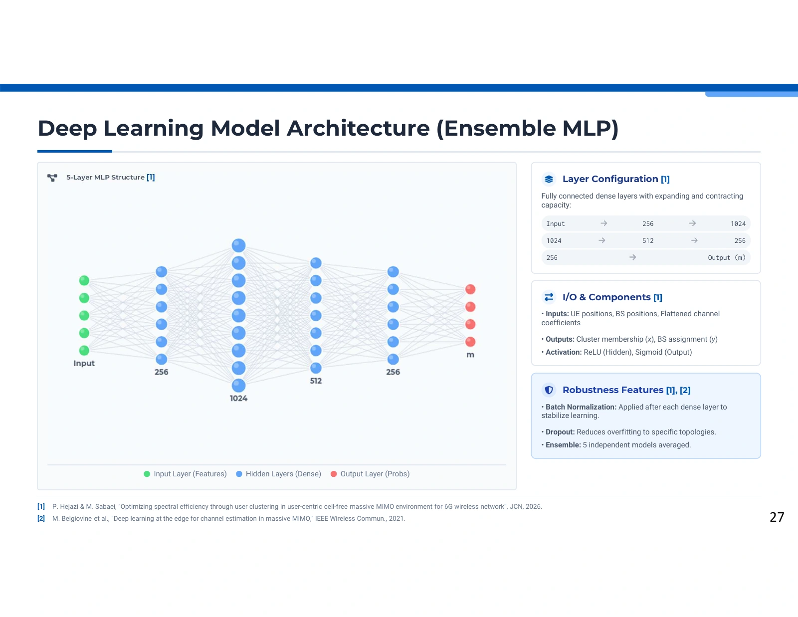
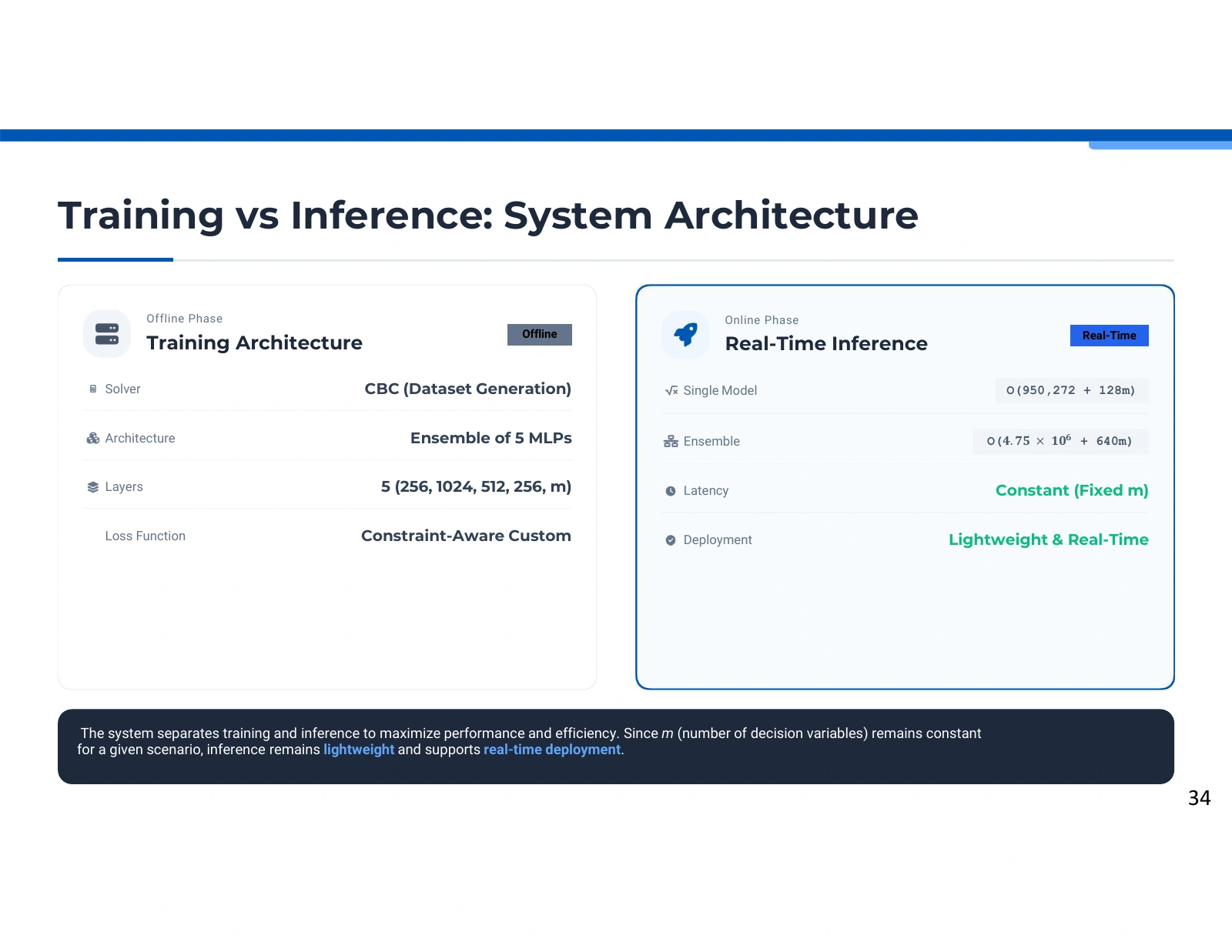
The neural architecture for allocation

A dense neural-network diagram connects input features through layers labeled 256, 1024, 512 and 256 to an output of size m, alongside notes on activations, normalization, dropout and ensemble prediction.
The neural architecture for allocation. Source: Pooya Hejazi’s research presentation. Open image to inspect.

A multilayer perceptron turns network features into allocation scores. Hidden layers model interactions, and output groups correspond to the different assignment decisions.

Representing a network instance

The inputs include user positions, base-station positions and channel coefficients. Flattening them produces a vector suitable for fully connected layers. Their ordering is part of the model definition: the same physical quantity must occupy the same feature position during training and inference. Normalization helps prevent differing numerical scales from dominating learning merely because of their units.

Read the full explanation

Hidden layers and output meaning

Dense layers combine features so that a prediction can depend on several users, links and resources together. The presentation illustrates expanding and contracting hidden widths, with ReLU activations, batch normalization and dropout. The final output has m components representing allocation variables, using sigmoid scores before the procedure interprets them as decisions.

Architecture versus a valid decision

The network structure explains how information flows through the predictor. It does not independently specify the ordering of every output variable or the rule for turning probabilities into a feasible schedule. Those details must remain consistent with the optimization labels. An ensemble can combine several predictors, but averaging cannot by itself impose the scheduling equalities and inequalities.

Technical details

  • The graphic is an architectural illustration, not a downloadable implementation.
  • The output dimension depends on the chosen network configuration and decision-variable layout.

Further reading: Paper 1, Section IV, PDF pp. 8-9. · Supplied presentation, Deep Learning Model Architecture.

User clustering

Teaching the predictor about allocation constraints

A composite loss expression combines weighted binary cross-entropy, a sum of penalties, user-association loss and base-station assignment loss; nearby panels explain the terms and adaptive weighting.
Teaching the predictor about allocation constraints. Source: Pooya Hejazi’s research presentation. Open image to inspect.

The training objective combines label-prediction losses with penalties for modeled allocation constraints. It encourages useful assignments while keeping feasibility a separately testable property.

Agreement with the labels

Classification losses measure how closely the predicted assignment scores match the optimization-generated targets. The user-association and resource-assignment outputs describe different decisions, so their losses preserve that distinction. Minimizing these terms helps the network imitate the label generator, whose decisions already depend on the source model's constraints and approximated objective.

Read the full explanation

Penalizing violations

Additional terms respond when predictions violate requirements such as membership, connectivity, pilot capacity or resource sharing. A weighted sum lets training trade prediction error against these residuals. The presentation describes increasing the penalty weight during training, aiming to give structural rules more influence as the predictor learns the basic assignment patterns.

Reading the word constraint-aware

A penalty makes a violation costly; it does not make that violation impossible. The final result depends on loss scaling, optimization, thresholds and how continuous scores become discrete decisions. Consequently, evaluating the method requires both prediction metrics and direct checks of the constraints on the resulting schedule. A small training loss is not equivalent to a feasible solution of the original optimization problem.

Technical details

  • Cross-entropy operates on classification targets; constraint penalties operate on relationships among the outputs and model inputs.
  • The displayed 1.1 multiplier describes the source's penalty schedule, not a general tuning recommendation.

Further reading: Paper 1, Section IV, PDF pp. 8-9, custom-loss discussion. · Supplied presentation, Constraint-Aware Loss Function.

User clustering

Combining several allocation predictors

Three explanation panels describe independent model training, averaging during inference, and the intended improvements in generalization and robustness.
Combining several allocation predictors. Source: Pooya Hejazi’s research presentation. Open image to inspect.

Ensemble learning combines independently trained predictors to reduce sensitivity to one model's errors. The resulting probabilities still need a clearly defined interpretation as allocation decisions.

Why models can disagree

Neural training depends on initialization and the examples encountered during optimization. Several models can learn slightly different mappings even when their architectures and objectives are similar. The presentation uses this variation as a reason to train multiple predictors, rather than relying on a single set of fitted weights for every network instance.

Read the full explanation

What averaging provides

The ensemble aggregates output scores for the same decision variables. Averaging can reduce fluctuations when individual errors differ across models. The components must share the same feature ordering and output interpretation, otherwise averaging combines unrelated quantities. Its benefit is empirical and depends on the diversity and quality of the component predictors, not simply on their number.

What remains after aggregation

An averaged probability vector is not yet a verified radio-resource schedule. Thresholding membership and resource scores can still create conflicting assignments or violate capacity and connectivity rules. Ensemble evaluation therefore includes the same questions as single-model evaluation: how accurately it matches labels, how well it preserves the objective and how often its final decisions satisfy all applicable constraints.

Technical details

  • Averaging predictions adds inference work roughly in proportion to the models evaluated, subject to implementation and hardware effects.
  • Claims about robustness should refer to the distributions and scenarios actually tested.

Further reading: Paper 1, Section IV, PDF pp. 8-9, ensemble and evaluation discussion. · Supplied presentation, Ensemble Learning Strategy.

User clustering

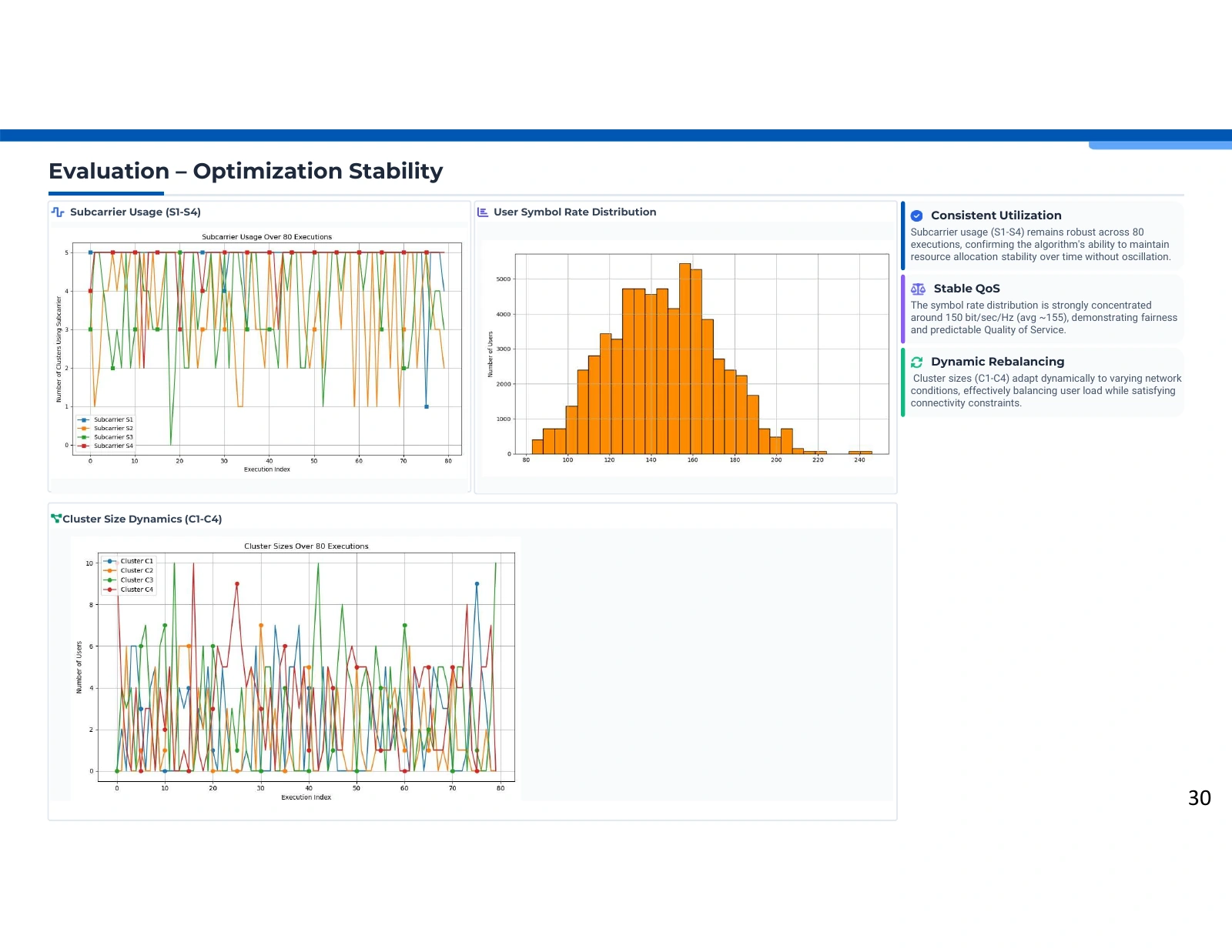
Reading resource use across optimization runs

Three charts show subcarrier usage across executions, a histogram of user rates, and cluster-size variation, with commentary about utilization, quality of service and rebalancing.
Reading resource use across optimization runs. Source: Pooya Hejazi’s research presentation. Open image to inspect.

Subcarrier usage, user-rate distribution and cluster sizes provide complementary views of the evaluated allocations. Together they show how the modeled resources and users are distributed across runs.

Resource utilization

The subcarrier chart tracks how often the available resources appear in the optimization outputs. Repeated use across runs indicates that the method is not relying on only one resource in the displayed sample. To interpret this correctly, the horizontal direction should be read as evaluated executions, not necessarily as a time trace from a functioning mobile network.

Read the full explanation

Distribution of user rates

The histogram shows where the modeled per-user rate values concentrate. The article reports a mean of 149.82 bit/s/Hz, with much of the distribution between 130 and 160 bit/s/Hz. A distribution is more informative than the mean alone because users can experience different allocations, but its meaning still depends on the study's rate model and selected scenarios.

Cluster sizes across instances

The cluster-size chart shows how the optimization distributes users among the available groups. Variation can reflect different geometries and channels, which is the intended reason for adaptive grouping. These plots support inspection of the reported outputs. They do not by themselves establish temporal convergence, a formal fairness property or a guaranteed quality of service for every user.

Technical details

  • Paper 1 groups these views in its optimization-stability analysis and Figure 5.
  • The presentation's approximate rate summary differs from the paper's reported mean; use the article's table and discussion for precise claims.

Further reading: Paper 1, Section III, PDF pp. 7-8, Figure 5 and rate-distribution discussion. · Supplied presentation, Evaluation of Optimization Stability.

User clustering

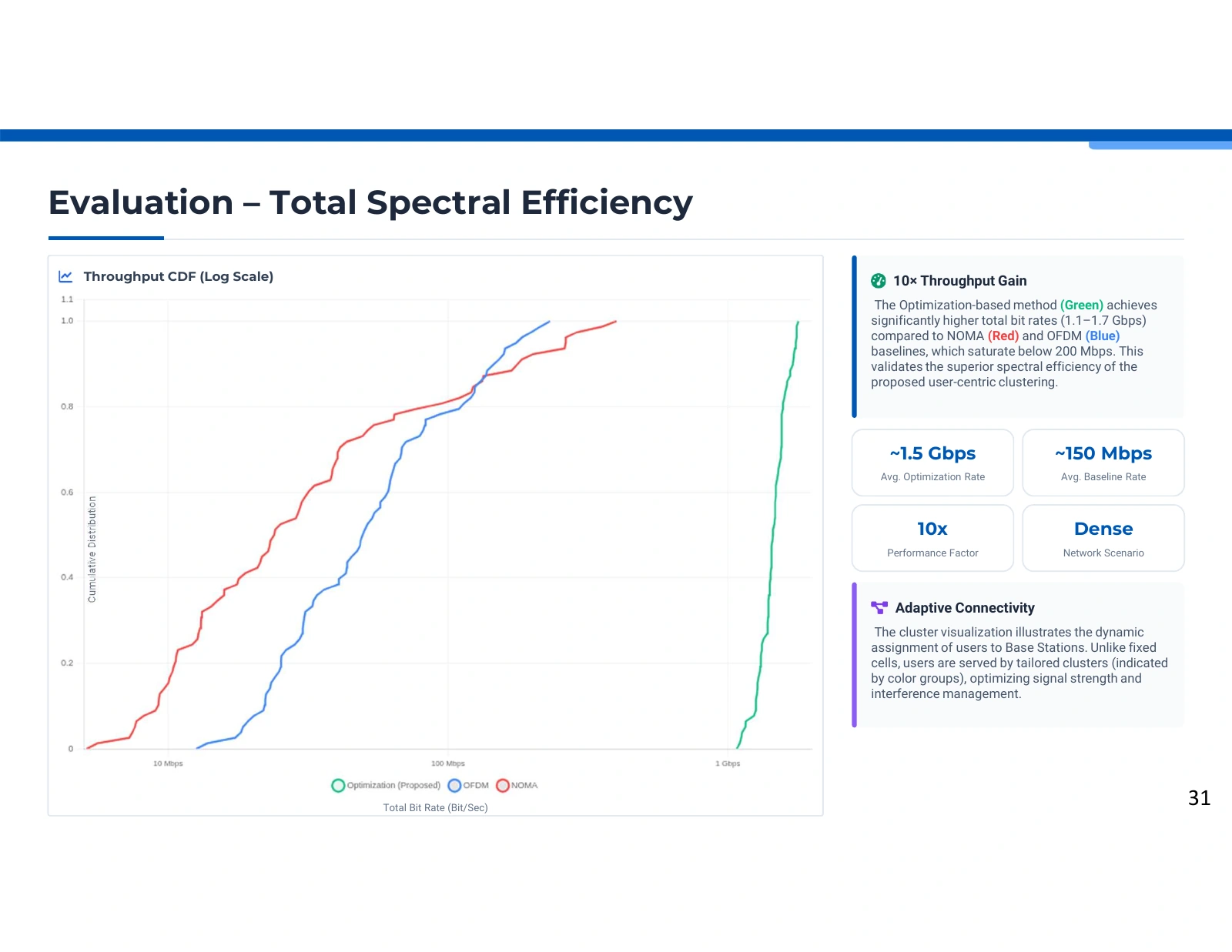
Comparing the distribution of total bit rate

A cumulative-distribution plot uses a logarithmic total-bit-rate axis and compares optimization in green, OFDM in blue and NOMA in red; adjacent panels summarize the source's throughput interpretation.
Comparing the distribution of total bit rate. Source: Pooya Hejazi’s research presentation. Open image to inspect.

The cumulative-distribution curves compare the reported total bit rates of optimization, OFDM and NOMA. Their horizontal separation summarizes a result within the modeled evaluation setting.

How to read the axes

For a chosen bit-rate value on the horizontal axis, the cumulative probability indicates the fraction of evaluated outcomes at or below that value. The logarithmic scale covers widely separated rates. Comparing the curves at the same cumulative probability gives a quantile comparison, which differs from comparing their means or the best observed outcomes.

Read the full explanation

What the displayed separation suggests

The optimization curve lies to the right of the NOMA and OFDM curves in the reported sample. This indicates larger total bit-rate values under the study's model and allocation procedure. The underlying explanation is joint user grouping and resource assignment, which can exploit modeled channel conditions more directly than the baselines being compared.

Keeping the metric precise

The horizontal axis is total bit rate, measured in bit/s. Spectral efficiency is a different quantity, normally expressed in bit/s/Hz. Converting between them requires a consistent bandwidth definition. The supplied paper gives differing bandwidth values in its setup and later discussion, so the website retains the source plot without converting it or deriving a new normalized metric from it.

Technical details

  • This is a distribution of study outputs, not measured commercial-network traffic.
  • A rightward CDF shift is a relative observation for the displayed experiment; it does not identify a universal multiplicative gain.

Further reading: Paper 1, Section III, PDF pp. 6-7, Figure 3 and bandwidth discussion. · Supplied presentation, Evaluation of Total Spectral Efficiency.

User clustering

Prediction accuracy and objective error

A result table reports 71.00 percent cluster-membership accuracy, 79.88 percent base-station assignment accuracy, 0.85 bit/s/Hz mean absolute error, and a source claim about constraint violation.
Prediction accuracy and objective error. Source: Pooya Hejazi’s research presentation. Open image to inspect.

The evaluation distinguishes matching cluster labels, matching resource assignments and approximating spectral efficiency. These metrics describe related but different aspects of the learned solution.

Two assignment tasks

Cluster membership identifies which group contains each user. Base-station assignment identifies how groups use serving resources. The reported accuracies are 71.00% and 79.88% respectively, so the predictor does not reproduce every solver-generated decision. Keeping the tasks separate makes it possible to see where agreement is stronger and avoids collapsing them into an undefined overall accuracy.

Read the full explanation

Agreement in the rate objective

The paper reports a spectral-efficiency mean absolute error of 0.85 bit/s/Hz relative to its optimization-generated targets. This is an error magnitude with units, not a classification percentage. Assignments that differ from a particular label can sometimes have similar objective values, so evaluating the rate alongside label accuracy gives a broader description of approximation quality.

Feasibility requires its own evidence

An accurate prediction can still violate a scheduling condition, and a feasible prediction can differ from the reference assignment. A feasibility statistic must specify which constraints were checked, how continuous outputs were discretized and what denominator defines the rate. The published headline metrics do not eliminate the need for these details, particularly when the model uses penalties instead of exact constrained decoding.

Technical details

  • The three article-backed values above come from Paper 1 Table II.
  • MAE describes average absolute error; it is not the largest error and does not certify all individual cases.

Further reading: Paper 1, PDF p. 9, Table II and Section IV evaluation discussion. · Supplied presentation, Evaluation of Deep Learning Accuracy.

User clustering

How channel-aware groups connect to base stations

Four spatial panels show colored user points, black cross-shaped base-station markers and dashed assignment links, accompanied by a topology legend and an explanation of channel-dependent grouping.
How channel-aware groups connect to base stations. Source: Pooya Hejazi’s research presentation. Open image to inspect.

Four spatial examples show users, base stations and assignment links. They illustrate the kinds of allocations produced by the modeled optimization rather than a rule based only on distance.

Reading the topology

The colored points represent users and the black crosses represent base stations. Dashed lines indicate the assignment relationships illustrated in each network instance. Colors connect the spatial positions to the cluster interpretation. The panels should be read as separate examples, rather than consecutive frames describing the movement of the same users.

Read the full explanation

Why the nearest station is not the whole story

The optimization incorporates channel coefficients together with resource and connectivity constraints. Distance contributes to propagation conditions, but it does not alone determine the best assignment under that model. Resource competition and the available channel gains can change which combinations serve the objective, so longer links in a drawing do not necessarily indicate an error in the modeled decision.

What the examples establish

The visualizations make the decision variables concrete: user membership and serving assignments become visible connections. They help a reader understand why a cell-free formulation can differ from a fixed nearest-cell partition. However, a handful of sample layouts cannot quantify generalization, mobility handling, handover behavior or the probability of satisfying constraints across every network instance.

Technical details

  • The sample layouts correspond to Paper 1 Figure 4.
  • The coordinate axes preserve the source's spatial presentation. Do not derive extra link budgets or distance-based performance values by measuring the image.

Further reading: Paper 1, Section III, PDF p. 7, Figure 4. · Supplied presentation, Cluster Connectivity Samples.

User clustering

Separating offline work from online prediction

Two columns compare offline CBC label generation and ensemble training with online neural inference, including single-model and ensemble operation-count expressions involving output size m.
Separating offline work from online prediction. Source: Pooya Hejazi’s research presentation. Open image to inspect.

Dataset generation and model training incur substantial offline work. Online inference evaluates the trained network, whose operation count depends on the architecture and output dimension.

What happens offline

The training side includes solving the allocation model to produce labels, preparing feature vectors and fitting the neural predictor. These costs contribute to the overall research workflow even though they are not charged to each later prediction. Repeating the workflow may be necessary when the scenario, input structure or operating distribution changes substantially.

Read the full explanation

What happens for a new instance

Online use passes the new features through the fitted network and interprets the output scores as allocation decisions. The displayed formulas separate a fixed contribution from a term proportional to m, the number of output variables. This explains why the cost can remain predictable for a fixed configuration without being independent of network size in general.

Operation count versus elapsed time

An arithmetic operation estimate is useful for comparing model structures, but it does not directly specify wall-clock latency. Hardware, precision, batching, memory movement and implementation affect runtime. Constraint checking or repair can add further work after prediction. The source's real-time motivation should therefore be read as a design aim supported by a complexity discussion, rather than an unconditional timing guarantee.

Technical details

  • The displayed ensemble expression scales the cost of an individual model by the illustrated number of models.
  • Changing users, clusters, base stations or subcarriers can change the number of decision variables and the feature layout.

Further reading: Paper 1, Section III.A and Section IV, PDF pp. 7-9, training/inference analysis. · Supplied presentation, Training vs Inference System Architecture.

User clustering

An upper bound from continuous relaxation

The formulation relaxes x, y and z from binary values to intervals between zero and one and connects the integer model, LP relaxation and Lagrangian dual with an upper-bound relationship.
An upper bound from continuous relaxation. Source: Pooya Hejazi’s research presentation. Open image to inspect.

Allowing binary allocation variables to take fractional values creates a linear-program relaxation of the linearized model. Its optimum can bound the integer model's achievable objective.

Enlarging the feasible set

Every feasible binary assignment also lies in the interval from zero to one. Replacing binary domains with these intervals therefore admits the integer solutions and additional fractional points. For a maximization problem with the same linearized objective and constraints, the relaxed optimum cannot be smaller than the integer optimum. That is the origin of the upper bound.

Read the full explanation

Why the relaxed problem is different

A fractional membership or assignment can be mathematically useful while lacking a direct interpretation as the original schedule. The relaxation provides an analytical benchmark, not automatically a realizable network allocation. The size of the gap between relaxed and integer objectives helps describe how informative the bound is for the particular model instance.

Duality at the correct level

For a feasible linear program with a finite optimum and the corresponding well-defined dual, strong duality relates the primal and dual optimal objectives. This equality concerns the continuous relaxation. It does not make the integer problem convex, remove an integrality gap or recover the original nonlinear rate objective that was approximated earlier in the formulation.

Technical details

  • The relaxation must consistently bound all relaxed variables, including auxiliary z variables, and retain the intended coupling constraints.
  • The inequality is an upper bound for the same linearized maximization model; an additional rate approximation needs its own interpretation.

Further reading: Paper 1, Section II.B, PDF pp. 5-6, underlying integer formulation. · Supplied presentation, Convex Relaxation of the MILP.

User clustering

Dual prices, threshold decisions and primal recovery

Four panels present coefficient-sign thresholding, the dual objective and multiplier domains, projected subgradient updates, and convergence conditions with a warning that raw Lagrangian maximizers may be infeasible.
Dual prices, threshold decisions and primal recovery. Source: Pooya Hejazi’s research presentation. Open image to inspect.

The Lagrangian separates relaxed variable decisions using multiplier-dependent coefficients. Iterative multiplier updates address constraint residuals, while feasible primal recovery remains a distinct step.

A simple inner maximization

When a relaxed variable t lies between zero and one and appears linearly as a times t, maximizing that term selects one if a is positive and zero if a is negative. If the coefficient is zero, every point in the interval maximizes the term. Separability allows this reasoning to apply to the variable groups after the chosen constraints enter the Lagrangian.

Read the full explanation

Learning the multipliers

The multipliers adjust the effective coefficients according to constraint residuals. Inequality multipliers are projected onto their permitted nonnegative domain, while equality multipliers are unrestricted in sign. The presentation describes diminishing step sizes and an outer minimization of a dual upper bound. The signs of updates must remain consistent with how each primal constraint and the Lagrangian are written.

Recovering a usable allocation

An inner maximizer can violate the coupling constraints that were moved into the Lagrangian. Dual progress therefore does not mean that every intermediate assignment is feasible. Averaging, projection or constraint repair may be needed to obtain a valid primal candidate, and binary scheduling requires further care. Stopping should consider feasibility residuals as well as changes in an objective value.

Technical details

  • The displayed convergence discussion concerns a feasible, bounded LP relaxation under the required algorithmic conditions.
  • A small change between successive dual values alone does not certify a feasible integer schedule.

Further reading: Supplied presentation, Lagrangian Dual Decomposition and Convergence. · Paper 1, Section II.B, PDF pp. 5-6, allocation model to which the discussion relates.

User clustering

What the clustering study contributes

A conclusion panel summarizes linearized allocation, optimization-guided neural prediction and reported spectral-efficiency results, with highlighted base-station assignment accuracy and mean absolute error.
What the clustering study contributes. Source: Pooya Hejazi’s research presentation. Open image to inspect.

The study connects a constrained allocation model with supervised prediction. Its contribution is the complete modeling-to-learning approach and its reported evaluation, within the assumptions used to construct it.

A structured allocation problem

User grouping and serving-resource assignment are modeled together, rather than solved as unrelated decisions. The formulation makes the relevant membership, connectivity and pilot conditions explicit. Auxiliary variables handle products of binary choices, while a rate approximation makes the objective suitable for the selected linearized optimization route.

Read the full explanation

A learned approximation

Optimization-generated instances become training examples for the neural predictor. The custom loss carries information about the assignment structure, and ensemble prediction is intended to improve approximation quality. The paper reports 79.88% base-station assignment accuracy and 0.85 bit/s/Hz mean absolute spectral-efficiency error, alongside the separate cluster-membership metric. These are conditional test results, not universal operating guarantees.

A practical interpretation

The intended advantage is to move expensive optimization work into preparation and use a trained model for faster predictions afterward. Evaluating that trade-off requires accounting for the approximation error, resource cost and feasibility of decoded decisions. Future use in a different topology or propagation regime would need validation rather than relying only on the performance of the original study's test instances.

Technical details

  • The physical scope remains the modeled quasi-static user-centric cell-free setting.
  • The reported rate histogram and label-prediction metrics answer different evaluation questions and should retain their units and definitions.

Further reading: Paper 1, Sections II-IV, PDF pp. 3-9, including Table II. · Supplied presentation, Part II Conclusion.
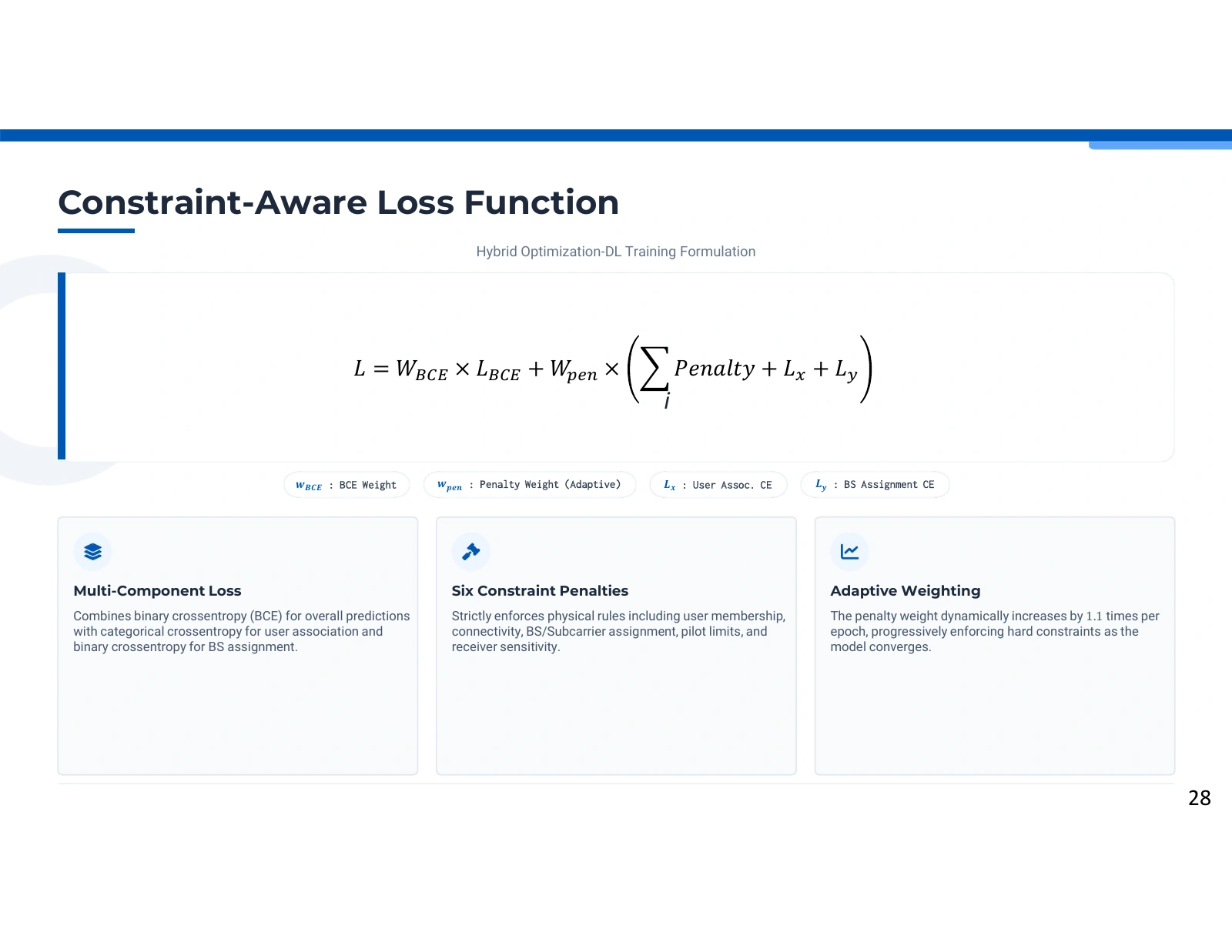
Synthesis

Channel knowledge and resource decisions

Three summary panels connect channel estimation, user-centric clustering and computational efficiency, with headline source claims about pilot savings and spectral efficiency.
Channel knowledge and resource decisions. Source: Pooya Hejazi’s research presentation. Open image to inspect.

The two studies address complementary parts of a wireless system: estimating its channels and deciding how users share serving resources. Their evaluations should remain distinct when presenting the combined research direction.

Estimating the physical channel

The channel-estimation study begins with received pilots and a least-squares estimate. A trained CNN refines that estimate, while GAN-generated data supports the training process. The central question is how to obtain useful channel estimates with a limited pilot budget under the evaluated ray-tracing conditions. Estimation error and inference cost are relevant measures for this component.

Read the full explanation

Choosing network assignments

The clustering study uses a constrained model to associate users with clusters and assign serving resources. Optimization-generated labels then supervise a neural approximation. Its evaluation concerns assignment agreement, objective error and modeled resource use. These measures operate at a different level from the channel estimator's NMSE and should not be merged into a single unspecified performance score.

Connecting the research questions

Better channel information can inform better allocation decisions, which makes the two directions conceptually complementary. A complete integrated claim, however, would require an experiment that propagates estimation errors into scheduling and measures the resulting system outcome. Presenting the studies together shows a research program without assuming that such an end-to-end deployment experiment has already been demonstrated.

Technical details

  • The GAN supports channel-estimator training; it is not an online allocation or channel-inference stage.
  • The two publications use distinct experimental configurations and assumptions.

Further reading: Paper 2, Sections III-IV, PDF pp. 3-6. · Paper 1, Sections II-IV, PDF pp. 3-9. · Supplied presentation, Summary of Contributions.

Synthesis

Lessons from combining models and learning

A synthesis page groups its message into data augmentation, hybrid modeling and future wireless readiness, relating LS plus CNN to channel estimation and optimization plus MLP to resource allocation.
Lessons from combining models and learning. Source: Pooya Hejazi’s research presentation. Open image to inspect.

The research uses mathematical structure to guide learning: a classical channel estimate anchors refinement, and an optimization model supplies allocation targets. Each hybrid design has a specific purpose.

Data generation shapes the result

The channel estimator learns from the distribution represented by its training examples. Ray tracing supplies structured channel instances, and GAN augmentation expands the training set. The quality and pairing of those examples matter as much as the number generated. Filtering examples also changes the evaluated population, so accuracy claims need to remain tied to the reported data-selection procedure.

Read the full explanation

Structure gives learning a role

The LS-to-CNN design gives the network a refinement problem after a classical initial estimate. The optimization-to-MLP design gives it an approximation problem after an explicit constrained label generator. These are different uses of learning, but both avoid requiring a neural model to define the entire physical or resource model implicitly from examples alone.

Evidence before generalization

The studies motivate further work on efficient wireless processing, but a favorable simulation comparison is not a universal statement that hybrid methods are always best. Hardware limitations, unseen environments, mobility and uncertain channels can change the trade-off. A useful lesson is to preserve interpretable structure while testing what the learned component adds under clearly stated conditions.

Technical details

  • Training data, optimization targets and validation cases are all parts of the method, not incidental preparation.
  • End-to-end network reliability requires more than a favorable estimator error or a prediction-accuracy figure.

Further reading: Paper 2, Sections III-IV, PDF pp. 3-6. · Paper 1, Sections II-IV, PDF pp. 3-9. · Supplied presentation, Key Takeaways.

Synthesis

Extending the questions to reconfigurable surfaces

Future-work panels describe RIS-aided channel estimation, generative methods for high-dimensional channel features, and joint phase-shift and clustering optimization.
Extending the questions to reconfigurable surfaces. Source: Pooya Hejazi’s research presentation. Open image to inspect.

Reconfigurable intelligent surfaces introduce controllable propagation paths and additional channel-estimation variables. The source proposes studying them as an extension of the existing estimation and clustering work.

A different channel structure

A surface-assisted link includes propagation through a base-station-to-surface path and a surface-to-user path. The effective channel also depends on how the surface is configured. Extending the existing estimator would therefore involve changing the channel model and data representation, rather than simply applying the same trained weights to a larger matrix without further study.

Read the full explanation

Learning with additional dimensions

The source proposes investigating generative or super-resolution approaches to represent the resulting channel features. This is a research direction motivated by the larger estimation problem. Establishing its value would require a suitable dataset, a defined observation model and comparisons that separate improvements due to additional training data from improvements due to architecture or sensing design.

Coupling propagation and allocation

Surface phase choices could be optimized jointly with user clusters and serving-resource assignments. That introduces additional coupling because changing a surface configuration affects the channel gains used by the allocation model. A convincing evaluation would need to account for estimation error, surface constraints and the cost of updating those settings alongside the resource decisions.

Technical details

  • The RIS material is a proposed extension, not part of the validated results of the supplied two main papers.
  • The external literature named in the image is contextual background; its findings are not relabeled as results produced by Pooya Hejazi.

Further reading: Supplied presentation, Future Work: Reconfigurable Intelligent Surfaces. · Paper 2, channel-estimation framework, PDF pp. 3-5; Paper 1, allocation model, PDF pp. 3-6, as starting points for the proposed extension.
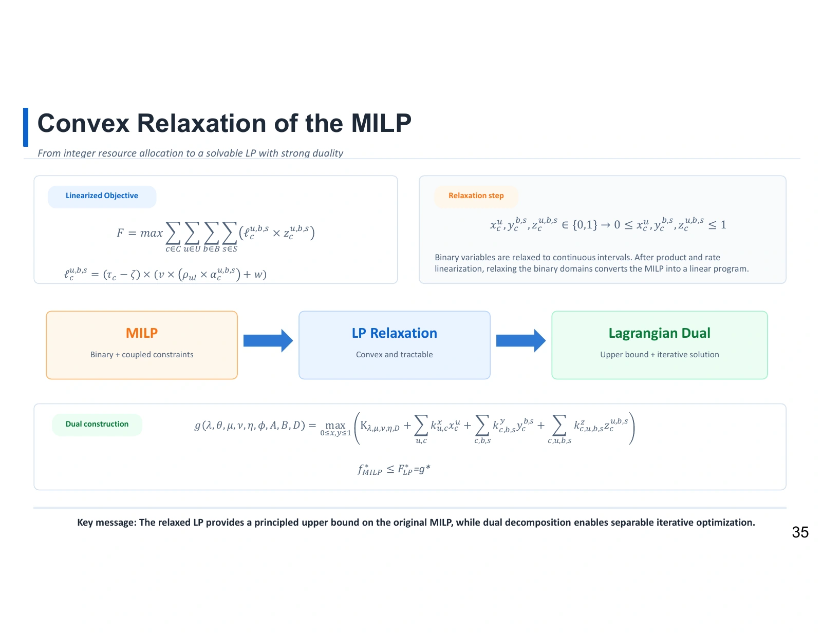
Synthesis

Exploring implicit models for channel refinement

Three future-work panels propose implicit-layer integration, memory-efficient training and physics-informed implicit operators for channel estimation.
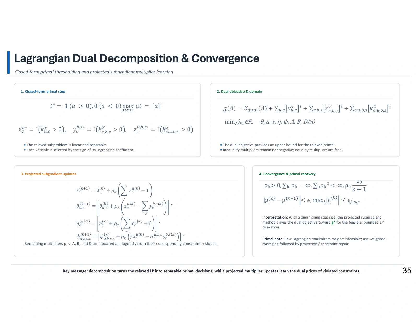
Exploring implicit models for channel refinement. Source: Pooya Hejazi’s research presentation. Open image to inspect.
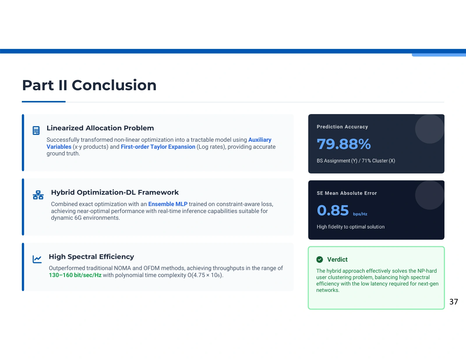
The source proposes replacing a fixed sequence of refinement blocks with an implicit representation defined through an equilibrium. This would change both model evaluation and training requirements.

A representation defined by a solution

A conventional network applies a fixed sequence of layers. An implicit formulation instead describes an internal state through an equation that must be solved, such as a fixed-point relationship. The source raises this as a way to explore adaptive feature refinement for channel estimation, rather than reporting that the existing LS-CNN model already has this architecture.

Read the full explanation

What must be evaluated

Solving for an equilibrium introduces questions about convergence, tolerance and computation per example. A favorable memory property does not automatically imply faster inference, because an iterative solver may perform different amounts of work on different inputs. Comparing this direction with the current CNN would require aligned data, evaluation metrics and a clear accounting of solver and training costs.

Adding physical structure

The presentation also suggests using channel properties inside the implicit operator. That could mean designing the learned refinement around an appropriate physical relationship, but the source does not specify a completed operator or validated constraint mechanism. The scientific opportunity is to investigate whether that structure improves generalization without making the solver unstable or excessively costly.

Technical details

  • The discussion is a future-work proposal inspired by the literature cited in the source image.
  • The existing channel-estimation paper supplies the LS/CNN baseline against which a new implicit model could be studied.

Further reading: Supplied presentation, Future Work: Implicit Layer Empowered Networks. · Paper 2, Sections III-IV, PDF pp. 3-6, current channel-estimation design and evaluation.
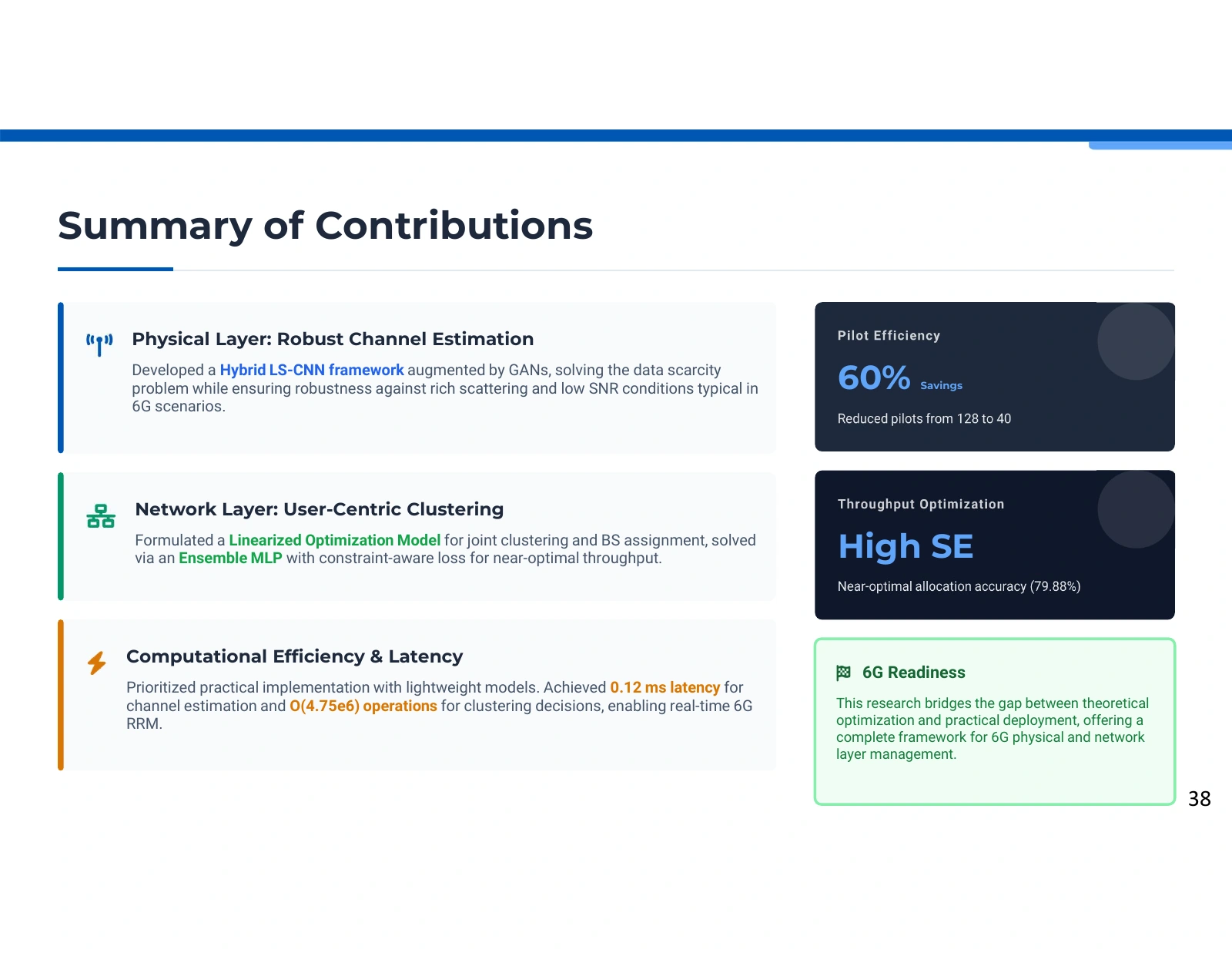
Synthesis

Mobility, changing channels and allocation updates

Three future-work panels discuss V2X mobility, dynamic channel tracking and temporal neural architectures for changing wireless environments.
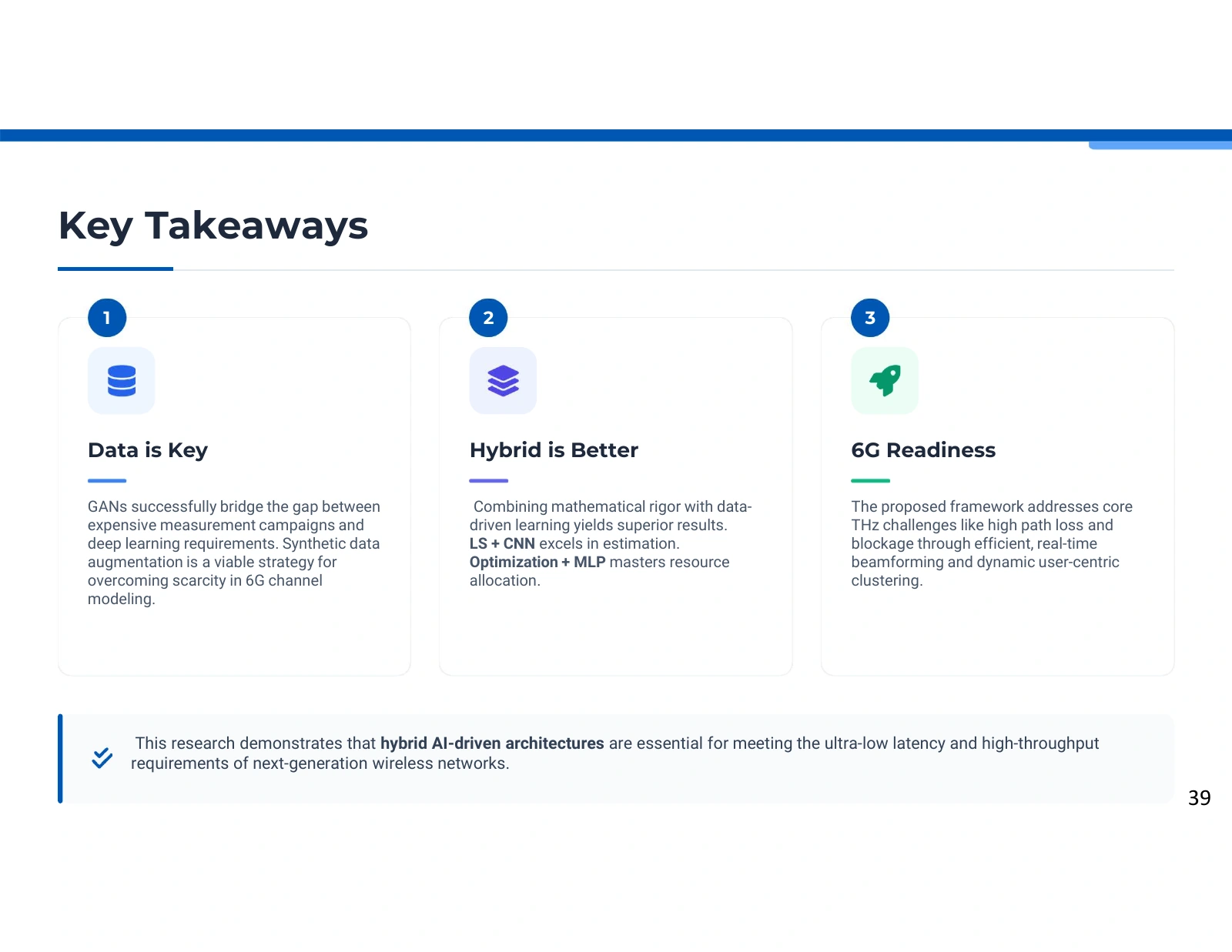
Mobility, changing channels and allocation updates. Source: Pooya Hejazi’s research presentation. Open image to inspect.

Moving users create a gap between the channel that was estimated and the channel used for transmission. The source identifies temporal tracking and dynamic allocation as future research directions.

Why the static assumption matters

The existing studies model quasi-static or slowly varying conditions. In a high-mobility setting, channel coefficients and useful serving relationships can change between observation and transmission. An assignment based on earlier information may therefore become less effective even if the predictor accurately reproduced the optimization labels for that earlier network state.

Read the full explanation

Tracking instead of one-shot prediction

The presentation proposes using temporal information to follow channel changes. Recurrent or temporal convolutional models are possible architectures for learning from sequences rather than isolated snapshots. A study would need to define observation intervals, prediction horizons and the source of sequence data before claiming that the model successfully handles Doppler effects or channel aging.

The cost of adapting the network

Reconfiguring clusters can improve alignment with current conditions, but it can also create signaling and handover costs. A mobile resource-allocation experiment should therefore evaluate how frequently assignments change and what happens during those changes. Throughput alone would not describe the whole trade-off; latency, continuity and the cost of acquiring fresh channel information would also matter.

Technical details

  • Vehicle-to-everything is an application direction mentioned by the source, not a deployment already demonstrated by the two main papers.
  • Any future temporal predictor should be evaluated with time-ordered data and a defined prediction horizon.

Further reading: Supplied presentation, Future Work: Mobility and V2X. · Paper 1, Section II, PDF pp. 3-6, quasi-static assumptions; Paper 2, Section II, PDF pp. 2-4, channel model.

Synthesis

The publication record behind the research

A publication list names the user-clustering article, the pilot-efficient channel-estimation article and an additional manuscript described in the source as submitted.
The publication record behind the research. Source: Pooya Hejazi’s research presentation. Open image to inspect.

The source connects the research narrative to its manuscripts. The website uses verified publication metadata for the two main articles and treats the additional submitted-work entry separately.

The clustering article

Optimizing Spectral Efficiency through User Clustering in User-centric Cell-free Massive MIMO Environment for 6G Wireless Network is the published source for the allocation model and its learning-based approximation. The website links its DOI, original PDF, conditional results and detailed method explanation.

Read the full explanation

The channel-estimation article

Pilot-Efficient Channel Estimation for 6G MU-mMIMO Using LS Initialization and GAN-Augmented CNN Refinement is the published source for the two-stage estimator. The supplied PDF is an accepted/early-access version, while the website's bibliographic record includes separately verified final issue metadata.

Status is part of the evidence

The additional joint-framework manuscript appears in the source as submitted. That label is a statement made by the source material, not independent confirmation of acceptance or publication. It is not counted as a verified published article in the website's main research index.

Technical details

  • Author lists, publication dates and final citation details should be read from each article's verified bibliographic record.

Further reading: Journal of Communications and Networks, published article records for DOI 10.23919/JCN.2025.000085 and DOI 10.23919/JCN.2025.000112. · Supplied presentation, List of Publications.

Synthesis

Questions and research discussion

A closing thank-you page invites questions and discussion and identifies Pooya Hejazi with his university affiliation and academic email.
Questions and research discussion. Source: Pooya Hejazi’s research presentation. Open image to inspect.

The closing visual invites questions about the research. The article pages provide the methods, original sources and limitations needed for a substantive discussion.

Discuss the method

Questions can focus on channel-estimation assumptions, the allocation formulation or the relationship between optimization labels and neural predictions.

Read the full explanation

Read the evidence

Use the linked article records for original PDFs, citations and study-specific results, including the caveats preserved in the detailed explanations.

Continue the conversation

The website's contact page provides the researcher's academic contact route for questions, corrections and collaboration.

Further reading: Supplied presentation, Questions and Discussion.

These are the author’s presentation materials and explanatory notes. Reported results retain their original study conditions; they are not newly reproduced experiments. Where a slide and its associated paper differ, the explanation identifies the discrepancy.